Table of Contents
iQ-Analyzer-X V1.11.1 Manual
This is the original, not translated, manual. It will be updated with every release of iQ-Analyzer-X. If you need to save the current version for some reason, please use the “Export to PDF” button. If you find anything missing or have suggestions, please let us know (support@image-engineering.de). We are happy to help!
The software is linked to this online manual. Click on “Online Help” and move the mouse pointer over the graphical user interface.

When you hover over a linked section, a question mark appears on your mouse pointer. Click on the section to go to the corresponding section in this online manual.
Please read the section Important Information about Test Charts to check, if special actions are required for the test chart applied!
What’s new in iQ-Analyzer-X?
The iQ-Analyzer-X is an all-new development. The most significant changes are:
- Increased overall speed (start-up time, detection times, etc.) due to the C++ implementation
- A versatile and customizable user interface
- Automatic chart detection and custom chart support
- Database storage for storing and accessing all previous results
- Custom workflows for managing unique evaluation specifications
- Side-by-side comparison of analysis results
System Requirements
The iQ-Analyzer-X is compatible with Windows 10 and 11.
Windows 11 on ARM (Apple) is also supported.
Limitation:
The automated chart classification depends on hardware-accelerated GPU support.
If this is not available on the PC, the chart classification is disabled.
As you might work with large image data files, please consider a PC with reasonable performance standards.
The iQ-Analyzer-X uses the industry-standard OpenGL for some 3D plots. Please be aware that such plots are not visible if the graphics board of your PC does not support OpenGL.
UTT users only: To import UTT reference files (.xlsx) to the iQ-Analyzer-X database, you need an installation of MS Excel or MS Office on the PC.
Licensing
The latest release of iQ-Analyzer-X is available to download on the Image Engineering homepage. If no dongle is attached to your computer, iQ-Analyzer-X runs as the Free Version with limited functionality. With an active license (via USB Dongle), the software will start as the Pro Version. If you have an active maintenance package, you can use all updates released within your maintenance period.
Free Version
- Compatible with all iQ-Analyzer-X test charts
- Install on unlimited devices
- Configurable user interface
- Analysis templates
- Analyze RAW files
- Configurable test result tables
- Zoom function of the image
Use individual reference dataSave results to a databaseExport results as XML or PDFMaintenance Package and Priority Support
Cultural Heritage Version
- Compatible only with UTT and Color test charts
- Install on unlimited devices
- Configurable user interface
Analysis templatesAnalyze RAW files- Configurable test result tables
- Zoom function of the image
- Use individual reference data
- Save results to a database
- Export results as XML or PDF
- Maintenance Package and Priority Support
Pro Version
- Install on unlimited devices
- Configurable user interface
- Analysis templates
- Analyze RAW files
- Configurable test result tables
- Zoom function of the image
- Use individual reference data
- Save results to a database
- Export results as XML or PDF
- Maintenance Package and Priority Support
Installation and Database Setup
To install iQ-Analyzer-X, click on the executable and follow the instructions. If you launch iQ-Analyzer-X for the first time, a local database will initialize for your analysis results. The progress of initialization is displayed in a progress bar.
Software updates are installed separately in their own folder. We recommend that you back up your database before updating the software, just in case something goes wrong. How to create a backup is explained in the “Database” section.
Note, that if you are considering using Open Database Connectivity (ODCB) in the future, you can use the “Database Migration Tool” to transfer the analysis data from a local to a remote server database. A migration from one to another remote database is also possible. The database migration tool can be started from the “Help” menu. It is explained in its own chapter.
Open Database Connectivity (ODBC)
iQ-Analyzer-X provides an interface for ODBC, enabling you to run a database on a remote server accessible from multiple PCs in different locations. To use ODBC, you need to create a database on your SQL server first. We have verified that MySQL, MSSQL, and MariaDB work well with the ODBC connectivity of iQ-Analyzer-X. Once you have created the database, you need to install the corresponding driver on your operating system. With the Windows “ODBC Datasources” tool, you need to set up the connection to the remote database. Note, that for MSSQL it is required, that the database you want to use is set as the default database in the database driver as well. If it isn't set, connection issues might occur.
After successfully connecting to the remote database, start the iQ-Analyzer-X and open the “Configuration” dialog. In the “General” tab is a section for the database configuration. Activate the “ODBC database” option. Now the dropdown menu for “Database name” is accessible. Choose the database you created from the dropdown menu. The database tries to establish a connection immediately and asks for your credentials. If it's the first time you connect to the database, you are asked to provide a “Network shared image folder” where all images are saved permanently. The folder can be changed any time in the settings. Also, you need to click on “Initialize database” to once set up the tables in the database. If everything worked correctly, the database status shows a green check symbol, and you are ready to use your database.

You can navigate to the “ODBC Data Sources” dialog by pressing “Configure Databases”.
Dongle
The USB dongle needs to be attached to your system to access the full functionality of iQ-Analyzer-X. The dongle keeps the information about your maintenance period, and the software shows a message before this period expires. Please contact our sales team if you want to extend the maintenance.
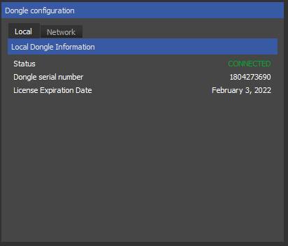
You can find general information about your dongle in the “General” tab under “Configure.”
Network License
A USB Dongle needs to be connected to the PC to run the iQ-Analyzer-X Pro Version. Since version 1.4, iQ-Analyzer-X also provides a network license feature. The USB dongle can be attached to a server, and the local PC does not need to have physical access to the dongle. With one USB dongle, you can have multiple concurrent with the network license. The management of the simultaneously running versions of iQ-Analyzer-X is performed with the help of user slots in a server file generated by the “MATRIX-Net” server program from “TechnoData Interware GmbH.”
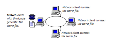
The MATRIX-Net functional principle is shown in the diagram above. The server program running on a computer with the dongle generates an encoded server file. Each running version of the iQ-Analyzer-X “connects” with the server file and occupies a user slot released when the application is closed. The network protection via MATRIX-Net does not use network protocols and can thus be used in any network system.
Installation of the Network License
When installing the network license, you need the mxnet32.exe, which is located in the installation directory of your iQ-Analyzer-X version under “NetworkLicenseTool.” Connect the dongle to your dedicated server and run mxnet32.exe. This process opens the MATRIX-NET program (the MxNet server application) and must run on the server PC.
The MxNet server program can also be registered as a Windows service so that the program is started automatically during the boot-up of Windows. The advantage of a service over an Autostart entry is the ability to start even if there is no User-Login in Windows. You can directly register MxNet as a service by starting MxNet with the corresponding parameters. The following call-up parameters are available: mxnet32.exe -i (Install MxNET service) and mxnet32.exe -r (Uninstall MxNET service).
After starting the MATRIX-NET program, a dongle symbol is displayed in the taskbar.

Clicking on this icon opens the MATRIX-NET dialog.
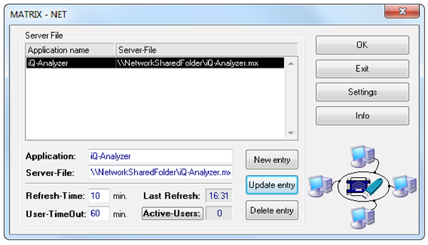
Create a new entry in the Server file list. Enter a name for the program in the field “Application name.” The name can be anything you like, and it does not need to match the actual application name. The network licenses are managed using a .mx server file. You can create the server file yourself and enter its path under “Server-File,” or you can enter a full path with a .mx file and click “New Entry.” The file is then automatically generated. The name of the server file must always be entered with the absolute path and correspond to the naming conventions of the operating system.
After setting up and running the MATRIX-NET server, install iQ-Analyzer-X on the client PCs. On each computer, you need to enter the server file you just created in the “Dongle File Path” field in the “General” tab under “Configure.” You can also browse for the file. After providing the path, click connect. If the connection was successful, the status is shown in green as “CONNECTED.”
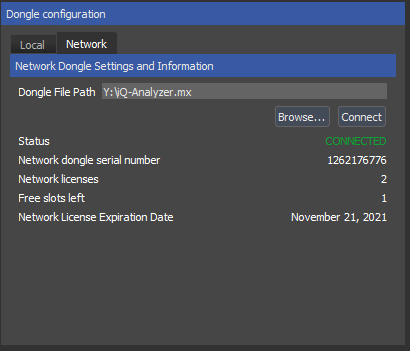
The “Network” tab shows information about the dongle, the total number of licenses, and the free slots.
MATRIX-NET Settings
REFRESH-TIME
In this field, the time interval for the refresh of the server file is set. The last refresh carried out is displayed in the “Last Refresh” field. The refresh period should usually be selected to be between 5 and 10 minutes.
USER-TIMEOUT
The User-TimeOut is the time limit after which the user is automatically removed from the server file. In the event of abnormal termination of the application (crash) on a client, this function ensures the release of the user slot in the server file, as this would otherwise remain occupied.
ACTIVE-USERS
This field is continuously updated and shows the total number of active users for the selected application. The “Active-Users” button allows you to display a detailed list of the active users. A user entry can be manually removed from this list. If your application is terminated abnormally on any terminal, you can either remove the user slot from the list or wait for the time out. When the user time out is reached, the user slot is automatically removed when the server file is refreshed. It is unnecessary to delete the user slot before the abnormally terminated application is restarted. The existing user slot will be found and refreshed automatically.
Important! Important! It is essential that the system time of the PC is synchronized in the network; otherwise, the “User-TimeOut” can not be correctly computed. The maximum allowed deviation of the system time between clients and server may not exceed the number of minutes selected in the MATRIX-NET server program in “Refresh-Time.” The following command can synchronize the clients’ system time with the server’s system time. This command can be implemented in the boot-up procedure of each client to make it an automatic function.
NET TIME \\<computername> /SET /YES
Getting started
This is a quick guide on how to run your first analysis in iQ-Analyzer-X Pro. If you use the CH Version, please refer to chapter “UTT”. Example images are provided on the iQ-Analyzer-X download page.
The first time you launch iQ-Analyzer-X it, takes a moment to initialize the local database in which the future analysis will be saved. After the initialization is done, click on “New Analysis.”

The “Import Images” dialog will appear. You can either load single images with “Open Image Files” or all the images in a folder with “Open Image Folder.” For now, please open a single image. The software detects the test chart automatically and shows it in the “Chart” column. If there are problems with the automatic detection, the chart can also be selected manually with the dropdown menu in the “Chart” column.
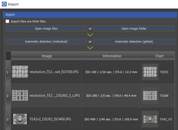
If all charts are detected, click “Import.” The main window will appear with the “Input“ dock showing the imported images.
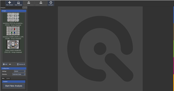
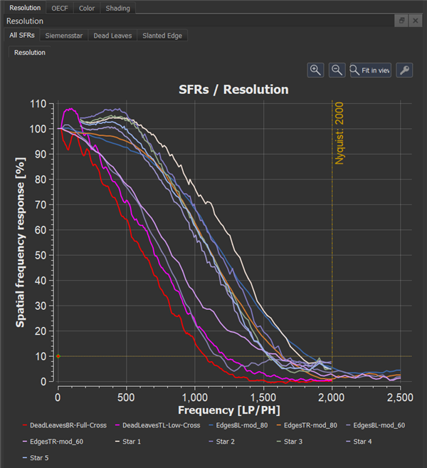
Apply your desired settings and the detection mode under “Configuration.” For your first analysis, the default values will be adequate. Click on “Start New Analysis” to launch the first image analysis. The results will be presented in the “Analysis results” tab when the analysis is completed. Switch through the different tabs to see the visualization of your measurements. You can also undock the tab from its container for a better view.
To save your analysis, click on “Save new analysis.”
Enter the details of your analysis and click on “Save Analysis.” A good description will help you find your analysis more quickly in the database.
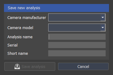
Congratulations! You just performed your first image quality analysis with iQ-Analyzer-X.
Important Information for Test Charts
Please check this list before working with your test chart. For most charts, we recommend to work with the individual reference file. Please refer to the chapter Reference Files for more information.
| Chart | comment |
|---|---|
| TE42LL 2AR | The chart comes with two reference files for the two different aspect ratios 4:3 and 16:9 which can be analyzed. Please assign the according .ref file in the “Import” dialog. |
| TE42LL | Only the corner and center Siemens Stars are analysed. |
| TE165 | Only the top row OECF patches are analyzed |
| TE188 | The default reference data is for reflective charts only. If your chart is transparent, it's required to import the individual reference file first, if available. |
| TE240 | The software only detects the chart, but not its variant (1:10.000 or 1:1.000.000). The default reference data is for a contrast of 1:10.000. If the contrast of your chart is 1:1.000.000 you need to create a reference file first! Please assign the correct reference data in the import dialog. |
| TE259 | Only the top row OECF patches are analyzed |
| All TE268 | From the slanted edges, only eight in the center are analyzed |
| All TE269 | The software only detects the chart, but not its variant ( A, B or C ). Please import and assign your individual reference file to avoid confusion. If you do not have an individual reference file, you need to import the default reference data of your chart first. The default reference files are located in C:\Program Files\Image Engineering\iQ-Analyzer-X X.X.X\resources\references\templates. How to import reference files is explained in chapter "reference files". |
| All TE264 | The software only detects the chart, but not its variant ( 10000:1 or 1000000:1 ). Please import and assign your individual reference file to avoid confusion. |
| TE296 | The chart is available in two contrasts, 4:1 and 6:1. A contrast of 4:1 corresponds to a modulation of 60% and 6:1 corresponds to approximately 70%. The graphs therefore show mod 60/70 in the legend. |
| All UTT Charts | An Excel Version needs to be installed to import individual reference files |
| iQ-Analyzer-X currently does not recognize the chart layout of the UTT (A0, A1, A2, A3 or A4) automatically. This means you need to assign the layout manually before analysis in the import dialog. A wrong allocation might lead to a crash. |
Image Quality Analysis
General Workflow
The iQ-Analyzer-X detects the type of test chart automatically and provides the results accordingly. The basic concept requires that each analysis is only for one specific device make and model. The analysis will be stored in a database, and several results of different cameras can be opened simultaneously for comparison. All necessary analysis settings are in one place, and you can create custom settings and store them in the database.
GUI Overview
The GUI consists of several docks and windows that can be individually placed on your screen by drag and drop. To change the position of a window, click into the top row and drag it to your desired position. If you drag it onto another window, it will show appear as a tab.
It is also possible to pin or unpin some of the sections by clicking on the small pin in the top right. An unpinned section will always be visible.

A pinned section appears as a symbol and can be unfolded by clicking on it. You can use this feature to get more working space.

You can always go back to the original state by selecting “restore view to default” in the “view” menu. Most result graphs and image overviews can be zoomed in and out with the mouse wheel or move positions with click and drag.
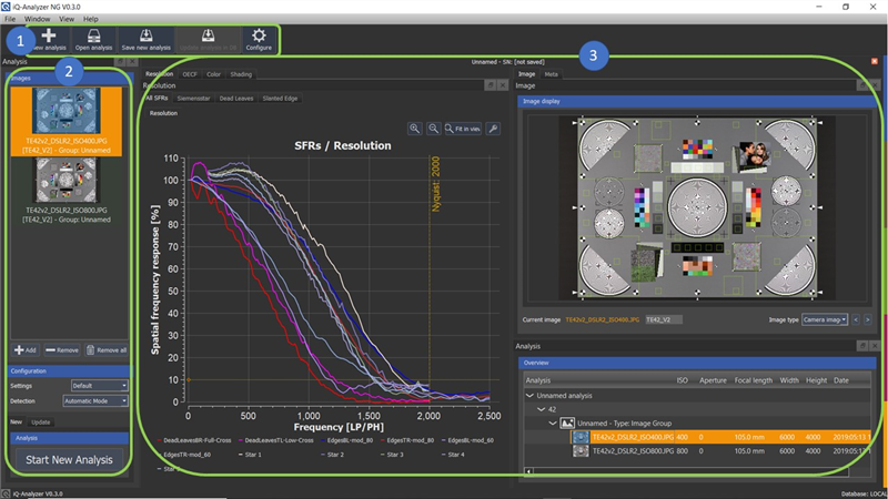
In the default view after an analysis, the GUI shows the “Toolbar” dock (1), the “Input” dock (2) (pinned), and the “Analysis Results” tab (3). The “Toolbar” provides a shortcut to a few basic functions. The “Input” dock shows all imported images and lets you define the settings for your image analysis. The “Analysis Results” tab contains all the results and information about the currently active test image. The currently active image is highlighted in orange.
Meta Tab
The meta information of the currently active image under test and analysis is displayed here. How to change the metadata is explained in a later chapter.
Media Tab
The current active test image or video with all ROIs detected is displayed here. This view is beneficial to check if the ROIs are in the correct location or any artifacts like reflections. It also highlights the corresponding targets when you hover over a line in its results plot. This feature makes it easy to see the target's connection and result. You can easily zoom in and out by using your mouse wheel, and the zoom will focus on the location of the pointer of your mouse.

Hover over the buttons below the viewer to see their functions.
Analysis Tab
This tab provides an overview of the images in your active analysis. If multiple analyses are open, the active analysis is the one with the highlighted text in the headline of its tab. The overview provides a simple way to switch between the test images or to show the results of multiple selected images combined in one plot and table.
Import Images
If you click on “New Analysis,” the “Import” dialog will pop up. You can either import multiple image files or an entire folder with images. iQ-Analyzer-X currently supports 8-bit and 16bit RGB images in *.tif, *.bmp,*.jpg, *.png format. For 16-bit RGB files, the images must not contain an alpha channel, and they require stating the actual sensor bit depth before import as, for example, a 16-bit image can contain 12-bit data. Some measurements depend on the actual bit depth to provide correct results. If iQ-Analyzer-X detects that the image you want to open is a 16-bit RGB Image, it opens the dialog automatically.

RAW bayer images in .tiff format and binary RAW files are currently supported with a bit depth of 8, 16 or 32 bit unsigned. If your images are RAW bayer, please refer to section RAW images
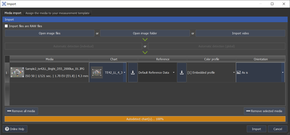
After opening the test images, they will appear in the “Import” dialog. If you have opened multiple image files, you can allocate the charts manually or automatically. Choose “Automatic detection” (individual) if the test images show different test charts and “global” if all images show the same test chart. To remove a test image, select it and click on “Remove selected images.”
If the chart detection doesn't work, the software will ask you to select the chart manually from the dropdown menu. The dropdown menu also shows “unknown chart” if this is the case. Note that if you want to analyze a custom chart, the automatic recognition won't work because it is not trained for custom charts. If this often happens, you can disable automatic chart classification in the “General” tab in the configuration dialog.
In the “Reference” Column you can select your reference file if you have one. For more information about reference files, please refer to chapter "reference files". You can also assign a color profile and rotate the image in this dialog.
Use the “arrow” button to assign your selection to the following images in the list.

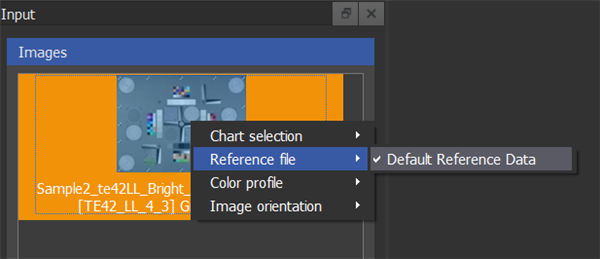
After the import you can still change these parameters for each image by right-clicking on the image in the input dock.
Note, that only specific test charts are supported by iQ-Analyzer-X. Please refer to https://www.image-engineering.de/products/software/iq-analyzer-x for details.
Most test charts will be delivered with a corresponding reference file (*.ref) or a *.pdf that contains your chart's individually measured data. The reference file can be imported in the “Reference files” tab from the “Configure” menu, and this reference file can be allocated in the column “Reference.” If you do not have a reference file, you can also allocate the “Default Reference Data”, which is less accurate and not recommended.
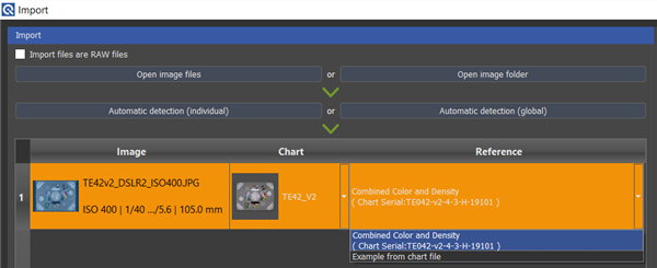
Please note, that if you have certain OECF charts, the software can only detect the layout and not the contrast or type of the chart. For example, if you import an image of the TE269 chart, the software cannot recognize whether it’s a TE269A, TE269B or TE269C. All of them have different patch densities. Therefore, you need to address the chart version by choosing the corresponding reference files in the “Import” dialog. This sequence also applies to chart TE264 and TE270. To do so, you need to import the default reference data of your chart first. The default reference files are located in C:\Program Files\Image Engineering\iQ-Analyzer-X X.X.X\resources\references\templates. How to import reference files is explained in chapter "reference files". If you purchased your OECF chart in 2024 it most likely has an individual *.ref file, which you can download here .
For greater accuracy, we recommend working with measured luminance when capturing transparent OECF charts. The reason for this is that when the chart is placed in the light source, it reflects into the light source, changing the output intensity.
Please refer to chapter "reference files" for information about creating and editing luminance reference files.
If all charts are adequately detected, and the reference files are also correct, click “Import.” The images will appear in the “Input” dock.
Raw Images
If your images are raw files, activate the checkbox “Import files are RAW files” before clicking “Open…”. In this instance, the following dialog for raw file import appears, where you can provide information about the raw file structure. Data formats supported are unsigned integer 8, 16 and 32 bit.

Width and Height: Image width and height in pixels.
Bits per color: Data format of the pixel values.
Header bytes offset: The number of bytes until the actual image data starts. It is important to get the correct starting point of the image data, so that the channel order is interpreted in the right way.
Byte Order: Choose between little and big endian.
Pixel Pattern: Choose the bayer pattern of your raw data, or apply “CUSTOM_4”.
Note, that the shown results depend on the pixel pattern. If you select “Custom_4” the OECF of all channels are shown, but no numerical results are calculated yet. However, you can export the results as .xml and in the .xml you can find the variance and the digital values for each channel and patch to do further calculations as, for example, SNR. If you choose a certain bayer pattern, a Y image is created. Y is a weighted sum of the channels and represents the perceived brightness. All numerical results are then based on this image. For RYCy-CFAs the channels are weighted equally. The Yellow channels are averaged before weighting. RGB-CFAs are weighted R = 0.2125, G= 0.7154 and B 0.0721. The green channels are averaged before weighting.
Bit offset: Images with metadata in a certain bit range can be imported with a bit offset. The bit offset is subtracted from all DVs. For example, if you have metadata in the first 8 bit, you can subtract 256 to get the real pixel value.
Sensor bit depth: The actual bit depth of the data. For example, 12-bit data in a 16-bit container.
If you have many differently structured raw files, you can save your settings for future analysis. To save a setting, you need to provide a name in the top dropdown menu. Once you have a name, the “Save” and “Save new” buttons are available. “Save” will overwrite your setting, while “Save new” will create a new setting in the database. You can access your saved settings via the dropdown menu.
Analysis Template (Image Sequence Analysis)
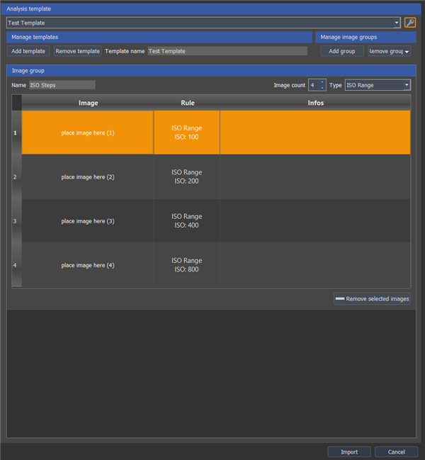
With analysis templates, image sequences with different apertures or ISO settings can be compared utilizing resolution evaluation. It is also possible to calculate the average of an image sequence or identify the image with the best resolution based on the MTF. You can create templates containing multiple groups, for example, one group for a range of ISO settings and one for a range of aperture settings. Templates are saved to the database and can be selected in the dropdown menu in the “Import” dialog.
Example ISO Sequence with three images:
We create a template for three images captured with different ISO settings in this example.
Click the key symbol to access the template settings.

Add a new template. Change the template name to “ISO Measurement Series,” for example.

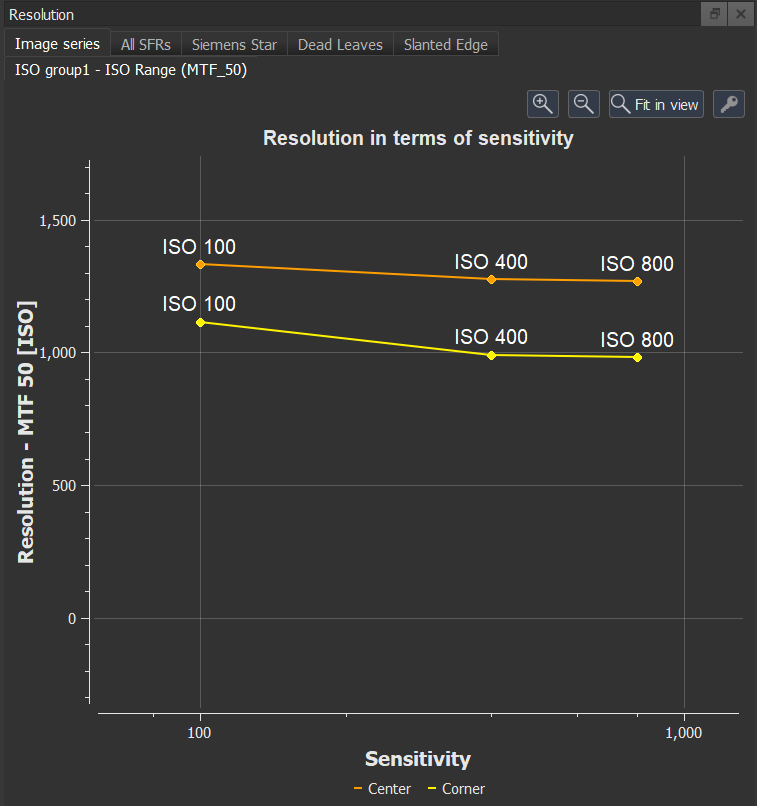
Name the Image Group “ISO group1.” Increase the image count to three. As “Type,” select “ISO Range.” Choose “MTF50” as measurement and “Center” as a group from the dropdown menu. The additional result plot then displays the MTF 50 values of the Siemens stars in the center over the ISO Range.

Change the ISO value in the column “Rule” to the corresponding properties of your images. In our case, it is 100, 400, and 800. You can change the value by double-clicking on the field and entering the ISO value.

After entering all ISO values, click on the key symbol again to leave the editing mode. Select the three images for analysis and move them to the placeholders.

Click “Import” after finishing the allocation of the images and analyze the images. A new tab will be added to “Resolution” called “Image Series,” which shows the MTF over the ISO value.
Average Measurement
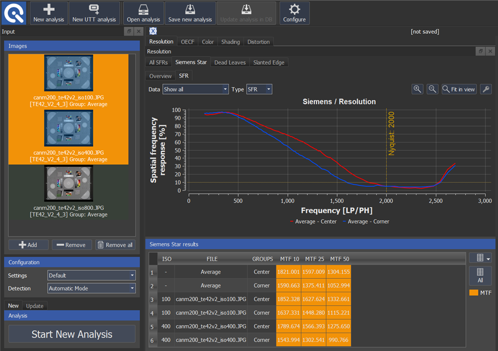
Measurement type “Average” can be helpful for measurements that have a significant variance due to the measurement setup. With this option, the average values of the numerical results are calculated, and the plots are adjusted. You can calculate the average of the whole image sequence or only a few images by selecting them in the “Input Dock.” In the following example, only two images are selected from the ” Average “ group, so the plots and numerical results show only the average of the MTF of these two images.
Best Of Measurement
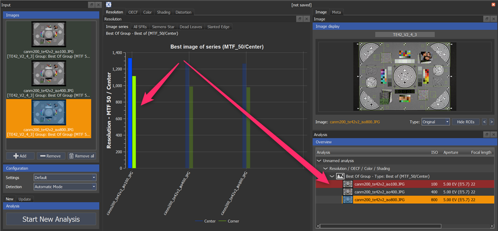
The “Best of” measurement determines the image with the best resolution based on the MTF. An additional “Image Series” tab is displayed, highlighting the image with the best performance. The image is also highlighted in the “Overview” area.
Analyze Images
All imported images are listed in the “Input dock” under “Images.” You can either add, remove or remove all images by selecting the image and pressing the corresponding button.
Under “Settings,” you can define the settings you want to apply to your analysis. You can change and save your analysis settings in the configuration tab under “Configure.”
There are two options for running an analysis, “Start New Analysis” and “Update Analysis.”

If you, for example, want to analyze the already imported images with different settings, you can update your analysis by pressing “Update Analysis.” You can also update the analysis with the already existing ROIs, modify the existing ROIs manually or start the automatic detection from scratch by selecting the appropriate item in the drop-down menu.
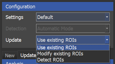
All results will be updated accordingly. Meanwhile, “Start Analysis” will create a new analysis in a separate tab. If you have two or more analyses opened simultaneously, the currently active analysis tab is highlighted with a brighter text.

ROI Detection
Under “Detection,” you can choose between three modes.
- Automatic Mode
- Semi-automatic Mode
- Manual Mode
In “automatic mode”, the software tries to find all ROIs automatically and analyzes the image immediately. In “semi-automatic mode, the software tries to find all ROIs automatically and opens the “Manual ROI Selection” dialog for further adjustments. In the “manual mode,” the ROIs are placed on the image independently of its content, and the ROI's sizes and positions depend on the principle layout of the assigned chart type.
Note, that automatic ROI detection relies on the image qualities like pixel count, noise, exposure, distortion, alignment of the chart,…
If not all ROIs were detected properly in “automatic mode”, the software asks you if you want to switch to “semi-automatic mode”, which opens the “Manual ROI Selection” dialog in which you can adjust the ROIs. The ROIs that need to be adjusted blink, to make it easier to find them. Note, that they keep blinking even if you changed their position.
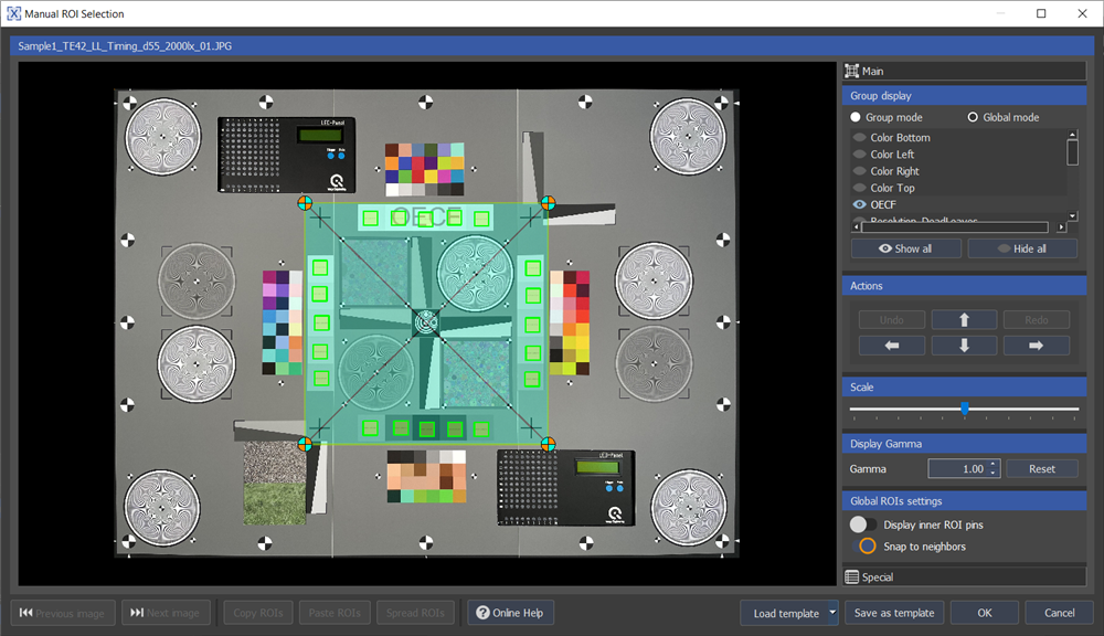
For captured images which do not show the chart full frame, you can use the “Crop and Detect” feature. The crop makes it easier for the software to find the ROIs in the image.
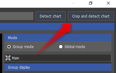
If you have a test image that contains multiple metrics, such as the TE42-LL, you can select the corresponding ROIs for one metric in the “Group Display” section. In “Group Mode” click on the entries in the list to turn them on or off. Once you have selected the desired ROIs, you can change their size and position. To change the size of a single ROI, for example, a color patch, activate “Display inner ROI pins”.

Then grab the ROI on its circle markers. Grab it in the center with a left mouse click and drag it to change its position.
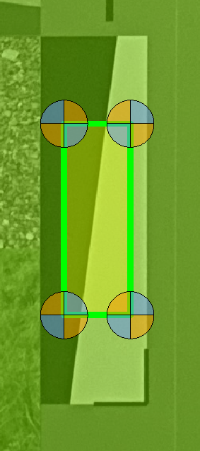
To change the position of all the ROIs of a single metric, you can use the pins at the edges of its surrounding container.
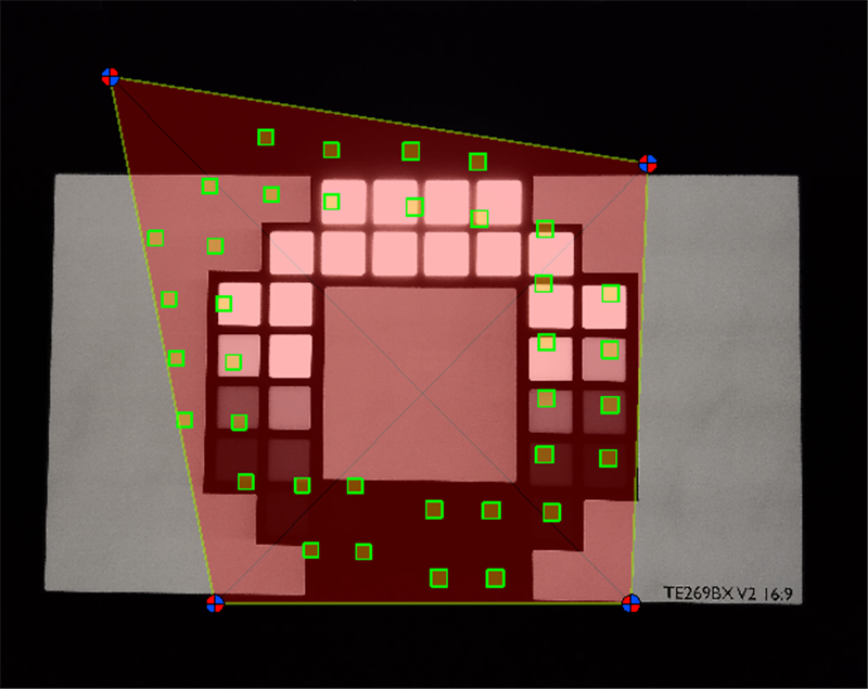
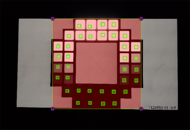
Use the “Global Mode” to change the position of all ROIs of all metrics in the chart at once. This adjustment moves all interior ROIs depending on their relative position to this box. It is useful if all the ROIs have an offset or are affected by distortion or misalignment.
If you only want to change the position of the ROIs, disable the handles by deactivating “Display inner ROI pins.” This option gives you a better view, and it is easier to drag the ROIs. When you enable “Snap to Neighbors”, a cross appears when the ROI is aligned with the center of a neighboring ROI.
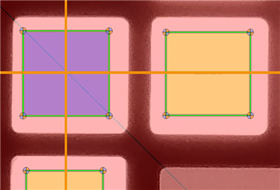
Select multiple ROIs with CTRL pressed.
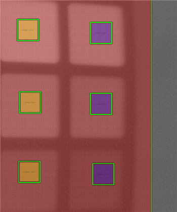
Or draw a rectangle to select multiple ROIs at once.
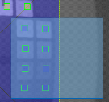
Especially if you work with HDR images, you might encounter that the images get very dark in the low light regions and the ROIs are not visible anymore. Change the gamma to make these parts brighter and adjust your ROIs.

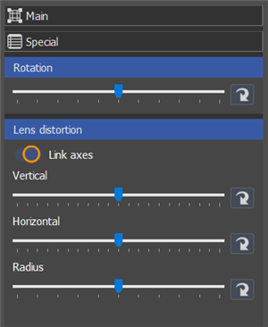
In the “Special” section, rotation or lens distortion can be compensated with the sliders. The sliders are only accessible, if “Global Mode” is activated, as lens distortion typically applies to all ROIs.
To get a better view, you can enlarge the size of the window or zoom in and out with the scroll wheel. If you have multiple test images with similar content, it's possible to copy the ROIs from one image to another. To do so, select the image which you want to copy the ROIs from with “Previous image” or “Next Image,” click on “Copy ROIs,” then select the image you want to paste the ROIs to and click on “Paste ROIs”.

If you're going to apply your adjustments to all images in the stack, click on “Spread ROIs.” With “Save as template” you can save the ROIs for an analysis in a new iQ-Analyzer-X session. Only one template per chart type can be saved. It can be loaded in the next session with “Load template”.
Load ROIs from previous analysis in the database with “Load ROIs from analysis”.

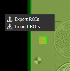
Its also possible to import and export ROIs from an analysis. Right-Click on the background in the “ROI selection” dialog to show both options.
If all targets are correctly detected, press ok to start the analysis. The results show up in the “Analysis Results” Tab.
How to draw the ROI for your target
Siemens stars
For all siemens stars, the center b/w marker should be approximately in the middle of the ROI.
If you are working with TE253 or TE268 siemens stars, the inner ROI should cover the entire star plus the surrounding b/w markers or the OECF patches.
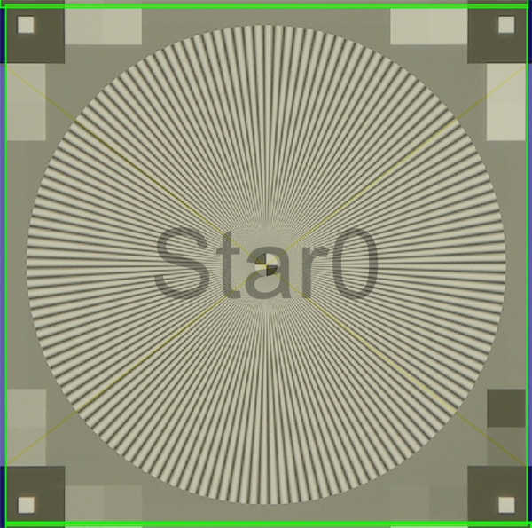
The ROI of the center star of the TE42V2 needs to cover the four black crosses surrounding it.
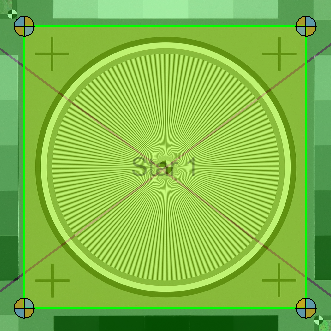
The ROI of the corner stars in the TE42V2 needs to cover the three big b/w marker.
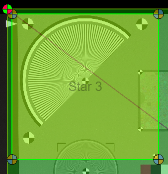
The ROI of the center and corner stars of the TE42LL needs to cover its surrounding four b/w marker.
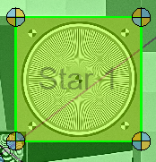
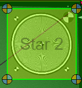
Note, that the ROI you set is only one of the steps for a proper detection of the siemens stars. Although you might have set the ROI properly, it can still be the case, that the star is not analyzed and shows no results. The “Error log” might help you find the reason for the failure.
Slanted Edges
The bigger the ROI for a slanted edge, the better the results. Depending on the image quality, you might be able to go down to 50px along the edge. The corners of the ROIs must have some distance to the edge.
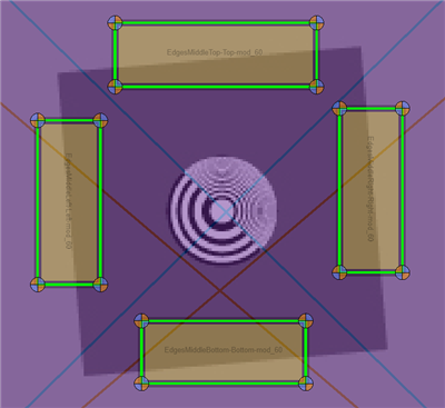
Dead Leaves
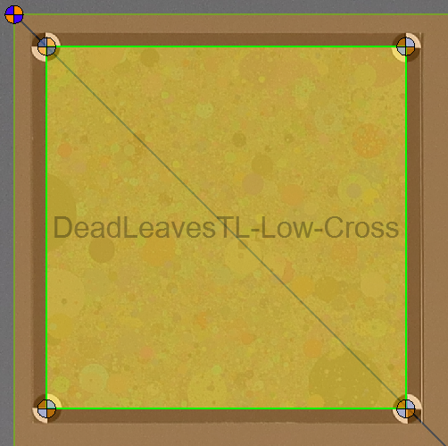
The edges of the Dead Leaves ROI needs to be approximatly in the center of the four corner b/w markers.
Error log
Warning and error messages regarding the analysis of the active session are output in the “Log”. You can open the log by pressing the red warning triangle on the bottom right. Once opened, the triangle will disappear, but you can always check the log under View→Show error log. Note, that the symbol only shows up in case there is important information for the user.
![]()
By default, clicking on “Log” in the bottom of the GUI will also show it.
A red message indicates a significant error, which might make the analysis or a part of it invalid. Yellow messages represent a warning. White messages contain general information.
Common Error Messages and Warnings
SFR Curve never falls below MTF
The SFR curve does not reach the required modulation before Nyquist frequency to calculate the desired MTF. This can, for example, happen, when a strong sharpening is applied or the resolution of the camera is much better than the resolution of the test chart. It might also appear, when the SFR results are too biased by noise or other artifacts. Is this the case, the MTF value reported is the Nyquist frequency with a negative sign.
ICC profile from image could not be loaded. Used default profile from settings
If iQ-Analyzer-X does not find a color profile in the metadata, it automatically applies the color profile, which is defined in the analysis settings.
WARNING: Example reference file for Color Analysis selected. Please use the appropriate reference file for your chart to achieve more precise results.
In this case, the default reference data has been assigned to the test chart. The default reference data is based on the target values, not the actual measured values. Depending on the type of analysis, it may make sense to work with measured color or density values, as they provide more accurate results.
Metadata
iQ-Analyzer-X automatically reads and displays metadata like exif data of the image if available. Under the media tab, the exif data is listed.
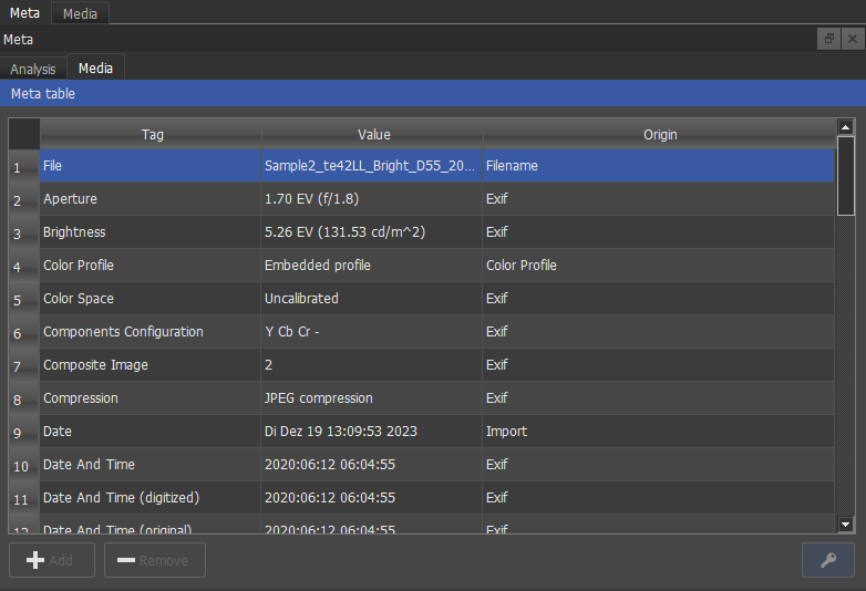
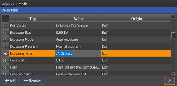
By clicking on the key symbol, you are able to modify it. To modify the data, double-click on the cell which contains the value you want to change. The changes will be saved with the entire analysis in the database. This can be useful if your DUT doesn't generate Exif data, but you want to document the settings like aperture, exposure time, etc. Also, for some result plots, the exposure in lux-seconds is calculated based on aperture and exposure time stated in the exif data.
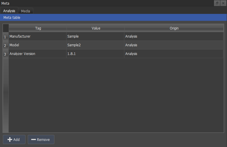
Under the “Analysis” tab you can add customized meta data like operator, test conditions or other. The meta data also shows upon the .pdf report and the .xml result file.
Save Analysis
Click on “Save new analysis” in the toolbar to save the results. Enter the information about the analysis in the dialog.

All fields except “Short name” need to be filled out to make the “Save analysis” button available. Note: If you want to compare two different cameras, you need to analyze each camera, and it is not recommended to mix the results of other cameras in one analysis. Once the camera model and make are saved with the analysis, they are available in the dropdown menu for future evaluations.
Open Analysis
Click on “Open analysis” to load an already existing analysis. In the “Open analysis” dialog, several filters can be applied to help you find your desired evaluation.

Comparison of Analysis
To compare two analysis, you need to save at least one of them first into your database. With the button “Append to view” in the “Open Analysis” dialog you can then integrate the results of the selected analysis to the currently active one.
Both analysis show up in the “Analysis Overview”. To compare the results, mark the images you want to compare with CTRL key and left-click. The plots and the numerical results now include these images.
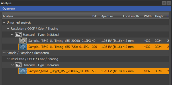
In some cases, when there are many targets in the image, the results can become confusing. To get a better overview, use the sorting function in the results table by clicking on the table headline or use the advanced plot settings. To enter the advanced plot settings, click the key symbol at the top of the plot.
Update Analysis in Database
To save changes in an already existing analysis, press on “Update analysis in DB” in the toolbar. You can still change the analysis name, serial number, and the short name in the upcoming dialog.
Delete Analysis from Database
To delete an analysis from the database, all analysis tabs in the current session must be closed, otherwise the Delete button will be grayed out.
Database
With the installation of the iQ-Analyzer-X, a local database is set up where all analysis results can be saved. You can also use a remote database, which is explained in this previous chapter. The database allocates a specific ID to every newly saved analysis. The ID is the main criteria for the database to distinguish between your analysis results. There can be two analyses with the same name but having different IDs.
It might happen, that the database needs to be updated when you update iQ-Analyzer-X. If it is required, you will be asked at program start, if you want to update the database.
We recommend that you back up your database before updating the software, just in case something goes wrong.
In the “Configuration” dialog under the “Maintenance” tab, you can see the currently used database and its version.

Here you can create or restore backups of your database and change the folder, where your database is located. To change the folder, click on the “Gear” symbol.

The database is a *.db file and by default the images are not stored in a backup. Check “Create backups including images” to include images. The symbol in the column “Type” shows, if images were included or not.
Database Migration Tool
If you started with a local database and want to copy your data to a remote ODBC or vice versa, you need the Database Migration Tool.
Start the Database Migration Tool from the “Help” menu.

To start the tool, close iQ-Analyzer-X.

In the dialog box that appears, select the source database on the left and the target database on the right. Enter your credentials if necessary. Finally, click “Start database migration” to start the process.

The progress is shown in the progress bar. When the migration is finished, a confirmation appears.

After confirmation, it still might take a few seconds to update the database information in the dialog with the new properties. At last the “Current source database content” and the “Current destination database content” should be equal.

Results
The results are provided numerical and in graphical representations. The plots that appear depend on the chart you are using. If you analyzed multiple images, the plots and the numerical results show the results of the marked image. To display the results of more images at once, select them using the Ctrl key.
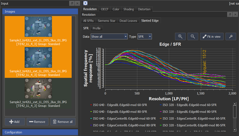
If a legend is shown with a plot, you can click on the legend to view or hide the legend's entries in the plot. Only Q1 and Q2 are shown in the graph in the example below, and all the other legend entries are hidden.
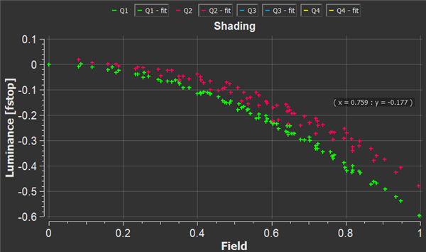
Zoom in or out of the plot using the mouse wheel. Change the plot's position by simply clicking and dragging.
The corresponding numerical results are shown in the table below the graphs. You can define the measurements you would like to include in the table by checking them in the dropdown menu on the right side.

Note, that not all parameters, shown in the list, are calculated. By default, the parameters, which are not calculated, are not checked in the list. These parameters do also not have any color coding. They have a gray background and show zero. Click on “Reset” to switch to the default measurements.

The results that belong together are marked in the same color. You can easily copy and paste the table to a spreadsheet software for further processing. Just select the cells you want to copy, or click on the top left square to select the entire table.

Or use the context menu which you can open by right-clicking a random cell.

Tip: You can sort the results in the table alphabetically or numerically by clicking on its headline. This way you can, for example, find the best MTF10 or compare two images in the rows next to each other.
Advanced Plot Settings
Some of the result plots offer advanced settings. You can access these options with the “Key” button on the top of the plot.

In the advanced settings you can adjust the scale of the X and Y-axis. Click on “Use manual scale” to activate the dropdown menus.

On the bottom of the plot some more options appear.

Channel: Depending on the chart and its metrics, you are able to choose between the R, G, B and Y channel.
Group by: Depending on the chart and the metric you are able to view the result of different groups. For example, Siemensstars on TE42 LL, if you choose the SFR Plot of the Siemens Stars, you can group the results by Segments, Stars, Groups or Image. Segments are parts of the Siemens Star, which is the smallest SFR measurement on a star. One segment is an eighth of a Siemens Star in a certain direction. “Stars” shows the SFR of the complete Siemens Star. “Groups” shows the center stars and the corner stars SFR separately. “Image” shows the average SFR of all Siemens Stars.
Tip: If you want to compare several images, mark them in the “Input Dock” and choose “Image” under “Group by”. Now you can see the average of all targets in each image in the plots and the results table.
Graphs: You can choose, if you want to see the “Mean of Selection” or each “Single Image”.
Unit: Choose the unit for the axis of the plot. For resolution you can choose between linepairs per picture height (LP/PH), linepairs per pixel (LP/PX) and linepairs per millimeter (LP/mm). For LP/mm you need to provide either the physical height of the sensor and its height in pixels or the pixel pitch. A dialog shows up when LP/mm is selected.
![]()
Legend: Define the position of the legend.
Resolution
Image resolution is the ability of a digital camera to reproduce the details of a scene. Resolution is an essential image quality attribute related to the overall image quality perceived by a human observer. Various factors influence image resolution, including the lens quality, alignment of the components, ideal focusing, exposure time, a sensor with optical components in front of it (low pass filter, IR filter, etc.), and aperture. All of these components are responsible for reproducing the details of objects within a scene.
iQ-Analyzer-X provides methods, each with different characteristics, to measure resolution. These include Siemens Star, Slanted Edge, Dead Leaves. The result in each case is a Spatial Frequency Response (SFR) or Modulation Transfer Function (MTF). Both designations are used equally in plots and numerical results.
For more information about the methods, please visit our homepage.
Another target for resolution measurement, currently only available for the TE42-LL UW, is the Tartan Target. This measurement is based on work within the VCX group and is still in beta status. A rough description of the method is in this paper:
VCX Version 2023 The latest transparent and objective mobile phone test scheme
Graphical Results
The MTF10 and Nyquist frequency are represented with the orange dotted lines shown in the graphs.
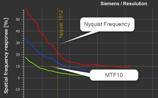
All SFRs
SFRs of all selected resolution measurements such as slanted edge, siemens star, or dead leaves are shown in one graph in this tab. If there are multiple targets for one measurement in the chart, the average will be displayed. The targets used for the results will be highlighted orange in the “Image” tab. Depending on the measurement, the curve might begin and end differently. A slanted edge SFR starts at frequency zero and ends above Nyquist frequency due to applied oversampling. The highest and lowest frequency of a siemens star is defined by the spatial frequency at the center marker and its circumference, and the dead leaves goes from zero to Nyquist frequency only.

Siemens Star
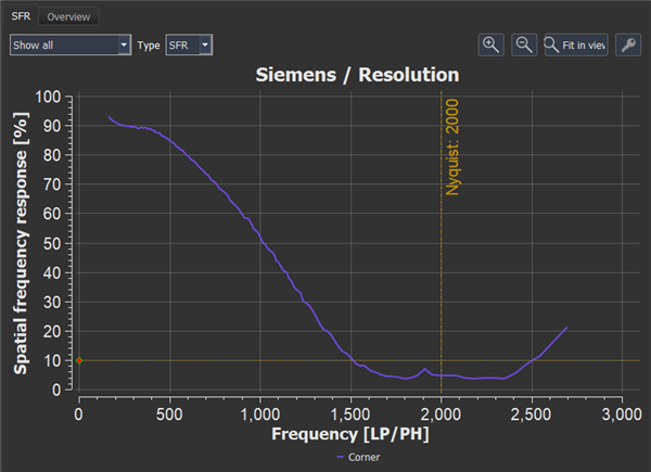
The SFR of a single Siemens star or all Siemens stars can be displayed in this plot. With “Type,” you can choose if the SFR is weighted with the viewing conditions to retrieve a vSFR and vMTF. The viewing conditions can be edited in the "Viewing conditions" tab. If you choose a vSFR, the graph's Contrast Sensitivity Function is added as a painted gray line.
Note that the plotted line of the MTF starts at the lowest frequency the siemens star can represent. The modulation at this frequency may not be 100%, depending on the quality of the camera system.
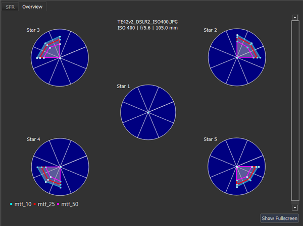
The overview shows a circle for every Siemens star in the chart, divided into eight segments. The image below shows the segment IDs. Please refer to the advanced plot settings if you want to see the MTFs of the single segments. The MTF10, MTF25, or MTF50 are calculated for each segment, giving you an excellent look at the resolution differences depending on the direction. The single circles show the percentage of how close the MTF10, MTF25, and MTF50 are to the Nyquist frequency. The circle's outline represents 100 percent of the Nyquist frequency, whereas the center represents zero percent. So the closer the MTFx curve is to the outline, the better.
The image below shows the IDs of the different segments.

Dead Leaves
For the SFR plot, please refer to "Siemensstar".
Slanted Edge
For the SFR plot, please refer to "Siemensstar".
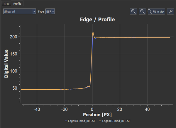
The “Profile” plot shows the edge spread function of the slanted edges in digital value over the position. The edge spread function plot is a valuable tool to identify sharpening in the image.
Tartan Target(Beta)
The Tartan Target is a pattern which consists of a certain number of spacial frequencies in tangential and sagittal direction. The Tartan Target analysis shows the SFR of the given spatial frequencies. Depending on the image quality, not all frequencies might be detected. The SFR between the frequencies is linearly interpolated.

Numerical Results

ISO: Shows the ISO setting of the camera, if available.
FILE: Shows the Filename.
GROUPS: If you captured a test chart with multiple targets, for example, the TE42 LL, targets might be grouped, and the results will show the group's average if you select “Show All” under “Data” in the graph.
EDGES: The identifier of the slanted edge.
MTF 10, MTF 25, MTF 50: The MTF values refer to the spatial frequencies that reach a particular modulation. For example, the MTF10 shows the spatial frequency that still reaches a modulation of 10%, whereas the MTF25 shows the spatial frequency that reaches 25% modulation. If the MTF curve doesn't reach such modulation until the end of the MTF curve, the MTF result shows the Nyquist frequency with a negative sign. Note, that the starting frequency and the length of the MTF/SFR curves depend on the measurement method. Slanted Edge and Dead Leaves always start at a frequency of zero, while the Siemensstar MTF starts at the lowest available frequency of the star. The Dead Leaves SFR is only calculated till Nyquist frequency. The frequency is expressed in LP/PH (line pairs/picture height) by default, but can be changed to line pairs per pixel or mm.
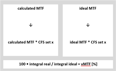
vMTF SET1-SET3: This measurement is similar to visual noise and quantifies how well a human observer can recognize noise. The vMTF (visual MTF) is also referred to as acutance! It implicates the three defined viewing condition sets. The calculated and the ideal MTF are multiplied with the contrast sensitivity function (CSF) and depend on the viewing condition sets for visual noise. The two integrals are divided. When multiplied by 100, you get the vMTF expressed in percentage.
Edge modulation: The modulation of the slanted edge in the linearized image. The value should be close but not necessarily equal to the modulation of the target.
Edge width (0-100%) and Edge width (10-90%) in px: The edge width is specified for 0-100% and 10-90% of the maximum modulation of the edge. It is the distance in pixel between two points in the edge profile with a certain modulation. The example below shows the edge width for 10 to 90%. The y-axis is the intensity in digital values for an 8-bit image from 0 to 255. The x-axis represents the position related to the edge. So, value 0 is the position of the maximum of the first derivative of the edge profile. For example, a value of 4 indicates that 4 pixels are right of the edge. Therefore, a value of -4 means 4 pixels are left of the edge. The left always represents the low intensity, and the right the high-intensity side of the edge.
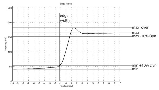
Maximum digital value: Indicates the average DV of the bright part of the edge.
Minimum digital value: Indicates the average DV of the dark part of the edge.
Overshoot and Undershoot: These metrics are calculated based on the edge profile and specify the undershoot and overshoot resulting from sharpening in the image. It is defined as (max_over-max)/max*100 for overshoot and the opposite way for undershooting.
Fit error (px): An ideal line along the edges has to be determined for the SFR-Edge approach. The fit error shows how well this line has been fitted into the real image data—the lower the value, the better the fit.
Tartan SFR(Beta): Is the area under the measured SFR. A value of one would mean that the SFR is at 100% up to the Nyquist frequency.
OECF
The Opto Electronic Conversion Function (OECF) can be determined with a grayscale target in a test chart. The OECF describes how a digital camera transfers the luminance of a scene into digital values in the image.
The test chart needs to be illuminated homogeneously to determine the OECF. In ISO 15739:2013, the digital value of the test chart background should be equal to 118. The OECF gray patches are also applied for Noise related and Dynamic Range measurements.
Most of the OECF plots have luminance, luminance(log) or exposure on the x-axis. Exposure requires the aperture and exposure time from the exif data to be calculated. If your plot shows only a vertical line, you may need to add these values to the Exif data in the Media tab under Meta. To do this, click on the key icon and then double-click on the corresponding entry.
Graphical Results
OECF + SNR plot
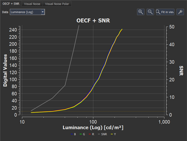
The OECF + SNR plot shows the optical-electronic transfer function and the SNR for the R, G, B channels, and Y. In the “Data” drop-down menu, you can define the parameter and scale for the x-axis. The SNR curve is the gray curve and its scale is on the right. The dotted red lines represent the lower and upper limit for DR calculation.
Note that even if the camera doesn't saturate, an upper limit is defined, which is the highest DV, and dynamic range (DR) is calculated. This DR value is then the minimum DR of the camera, but not the maximum DR. This basically means that if “Saturation reached” = 0, the minimum DR is shown in the results, if “Saturation reached” = 1, the maximum DR is shown in the results.
If the camera doesn't saturate, check if the chart contrast is suitable for the device under test and if the exposure was set correctly.
Visual Noise
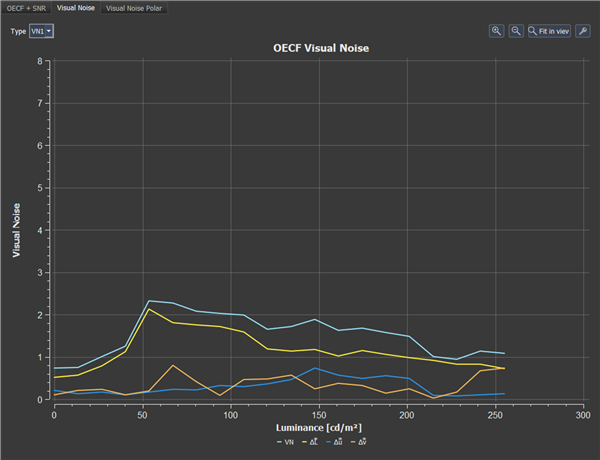
The visual noise graph shows the visual noise determined over the luminance values according to ISO 15739. The curves named Delta L*, Delta u*, and Delta v* show the share of the individual parameters to the overall visual noise. The visual noise depends on the viewing condition set in the configuration menu. You can exhibit visual noise for the three viewing conditions (VN1, VN2, VN3), with the “Type” drop-down menu in the upper left corner.
Visual Noise Polar
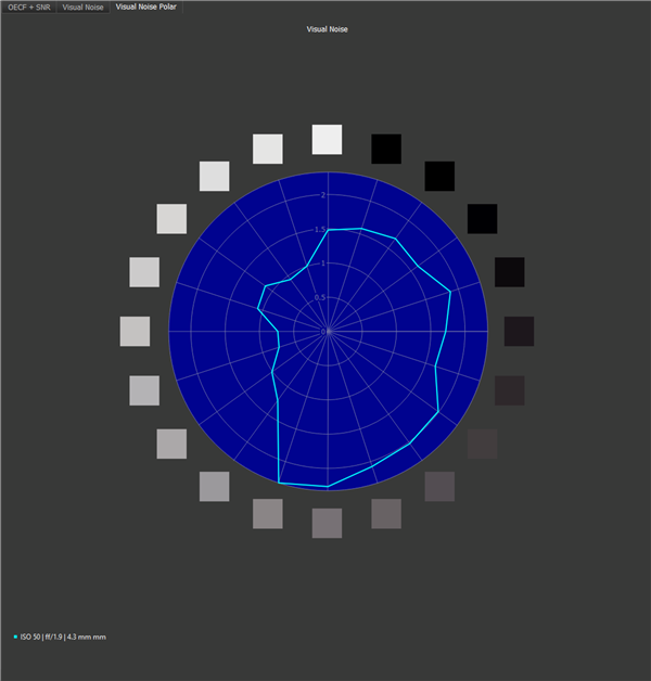
Visual Noise Polar: The polar plot shows the visual noise over the gray patches in circular arrangement. The patches are sorted by number, from first to last patch. The brightness of the patches is determined by their gray value in the test image.
Incremental Gain/Sigma Total
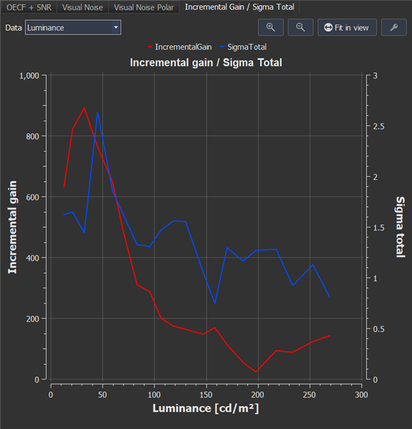
Displays the incremental gain and sigma total values for each OECF patch.
Numerical Results
OECF+SNR
SNR is defined as the ratio of the signal value to the standard deviation of the signal value. iQ-Analyzer-X calculates a Y (luminance) image and uses this for further calculations. The results are also indicated as digital values [DV]. The following calculations are based on ISO 15739:2013 which is currently applied in iQ-Analyzer-X. For the chart-based OECF, the reference luminance (Lref) shall be determined as the luminance corresponding to a digital level of 245 (for sRGB 8 bit) on the OECF function. For a more detailed description, please refer to the ISO paper.
LREF: Luminance corresponding to the digital value of 245
RREF : Log luminance value at the reference luminance.
S-1: The inverse of the camera OECF curve, S
I: digital value = 245
SNR total: Total noise means all unwanted variations captured by a single exposure.
Total standard deviation: Standard deviation of the total noise for a single image and multiple images when analyzing “n” images.
The signal-to-noise ratio is determined by:
SNR Total (dB): SNR TOTAL is specified in dB.
Mean Visual Noise: The numerical value for Visual Noise is a weighted sum of the standard deviation of each channel in the CIE-Luv color space. To give further insight into the noise characteristics, we also provide the visual noise metric for all three viewing conditions, which can be specified in the settings. In the results table the visual noise measurements are color coded.

Max Visual Noise: The maximum visual noise.
Mean ΔL*: Mean standard deviation in CIE L*.
Max ΔL*: Maximum standard deviation in CIE L*.
Mean Δu*: Mean standard deviation in CIE u*.
Max Δu*: Maximum standard deviation in CIE u*.
Mean Δv*: Mean standard deviation in CIE v*.
Max Δv*: Maximum standard deviation in CIE v*.
Dynamic range: The dynamic range is provided in f-stops, densities, and dB. It applies to ISO 15739:2013. The ISO DSC (Digital Still Camera) dynamic range is the ratio of the maximum unclipped luminance level Lsat to the minimum luminance level that can be reproduced with a signal-to-noise ratio of at least 1, Lmin.
Note that even if the camera doesn't saturate, an upper limit (Lsat) is defined, which is the highest DV, and dynamic range (DR) is calculated. This DR value is then the minimum DR of the camera, but not the maximum DR. This basically means that if “Saturation reached” = 0, the minimum DR is shown in the results, if “Saturation reached” = 1, the maximum DR is shown in the results.
If the camera doesn't saturate, check if the chart contrast is suitable for the device under test and if the exposure was set correctly.
The default threshold is SNR=1.
If the threshold cannot be reached, a 2.0 density “black reference” calculates the dynamic range to avoid black level clipping problems.
The value for Lmin shall be calculated as
σtotal (2.0): The black total noise measured at a density of 2.0.
Color
Camera color characterization is an essential step in the color image processing pipeline. It evaluates how the camera module translates RGB raw data from the sensor to the desired color space. Improper color calibration and characterization can lead to false-color reproduction, thereby hurting an image's overall image quality. The color reproduction is usually described with the Delta E metric, which represents the color difference of the color in the test image to its reference color. Note that there are different formulas for the calculation of Delta E. Therefore, you also need to state the applied formula.
Graphical Results
Delta Tables

The “Delta tables” tab shows a color-coded square for each color patch in the test image. These squares also exhibit the numerical parameter value selected in the drop-down menu. You can choose between Delta E, Delta E_ab, Delta L, Delta C, Delta H, and Visual Noise. The scaling of the color coding can be adjusted under “Visualization” in the “Configure” dialog.
“Visual Comparison” compares the color in the test image and the color of your reference.
Delta 3D Plots
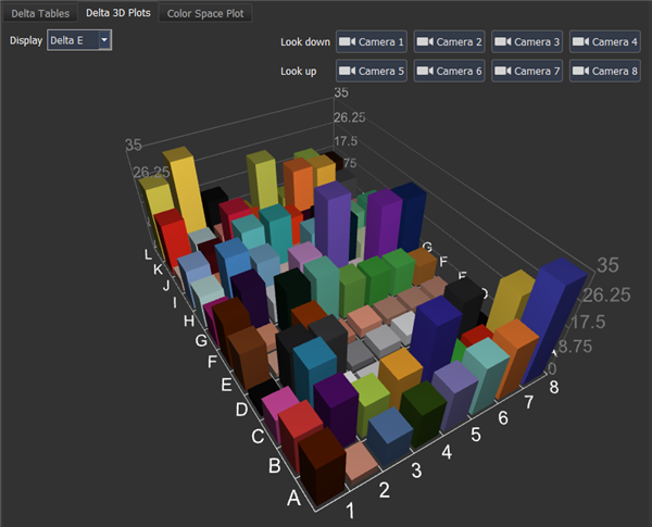
This plot shows the Delta values in 3D bars. You can change the perspective by using the different camera positions or dragging the plot with your mouse. In case of negative values, it makes sense to use the bottom camera views.
Color Space Plot
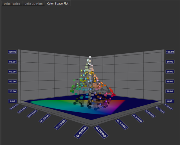
The calculated colors of the image and the reference are displayed in the CIE xyY color space, where x and y are the chromaticity coordinates, and Y is the luminance. The colors of the image under test are represented by a sphere and the reference colors by a cube. Click on the geometries to see its CIE x, y, and Y values.
Numerical Results
The mean and maximum values are stated for different groups, defined in the reference file. A group can, for example, contain only the skin, color, or neutral tones. “General” groups all patches.
Delta E: The iQ-Analyzer-X calculates Delta E from two Lab data sets, the reference, and the image sample set. You can choose between four Color Difference Formulas for calculating Delta E under “Analysis Settings,” with the most common calculation being CIE1976.
CIE1976:
If you express the Lab in polar coordinates, you get LCH, where L is the luminance, C the chrominance, and H the hue. Delta E indicates the overall difference between reference and sample. It might also be interesting to look at the difference between Luminance Delta L and Hue Delta H to get more detailed information about the deviation.
CIE1994 is calculated based on the CIE LCH color space and includes weights for Luminance, Chroma and Hue to address perceptual differences.
CIE1994:
In iQ-Analyzer-X, the following parameters for graphics and photography are used.
kL = kC = kH = 1
SL = 1
SC = 1 + 0.045 Csample
SH = 1 + 0.015 Csample
CIE2000:
Compared to CIE1994, the rotation term is added as the fourth element and only takes effect in the blue region.
CIE2000 SL1:
The same formula as CIE2000 with the factor SL set to 1.
Delta E_ab: Delta E_ab is similar to Delta E but doesn't take the Delta in luminance, into account.
Delta L*: Delta Luminance is based on CIE LCH color space and represents the difference in luminance.
Delta H*: Delta Hue is based on CIE LCH color space and represents the difference in color.
Delta C*: Delta Chrominance is based on CIE LCH color space and represents the difference in color saturation.
VN SET1-3: Visual Noise is described in ISO 15739. It correlates much better with the human perception of noise than a standard SNR measurement, and is stated for three viewing conditions.
Shading
The shading results show how uniform a camera reproduces a test image of a flat field, meaning a surface with uniform intensity. This test can be an image of a uniform test chart like the TE255 or an image of a light source with a uniform opening like the CAL series.
Please note, that currently, no linearization is available for the shading analysis.
Graphical Results
The plots offer different metrics for Shading, Color Shading and Noise which can be selected in the dropdown menu.
2D plot
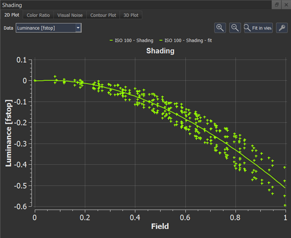
The “2D plot” shows the shading measurements over the field of the test image. The field is a line drawn from the center of the test image to the corner, with the image center being field=0 and the corner being field=1. All shading ROIs are mapped to the field along their radius.
Color Ratio
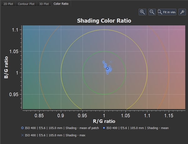
The “Color Ratio” plot shows the ratio of blue and red over the green channel and is, therefore, suitable to show color shading in the image.
- “Shading - mean of patch” is based on the average ratio in a single patch.
- “Shading - mean” is the average of all B/G and R/G ratios.
- “Shading - max” is the maximum of all B/G and R/G ratios.
The green, yellow and red line circle do not refer to any standard and are only for orientation. They circle around the ideal color ratio of one in 0.05 steps.
Visual Noise
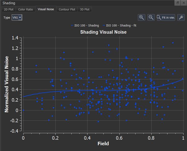
This plot shows the Visual Noise in the shading ROIs over the field for the viewing conditions which are defined in the analysis settings. You can change the viewing condition by selecting VN1, VN2,…from the dropdown menu.
Contour plot
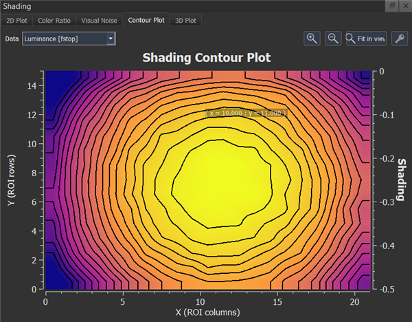
The “Contour” plot shows the uniformity over the columns and rows of the ROIs as an interpolated color-coded image. The contour lines are automatically fitted between the “minimum value” and “maximum value,” these can be changed under “Visualization.” The scaling of the color coding can be changed in the “Visualization” settings.
3D Plot
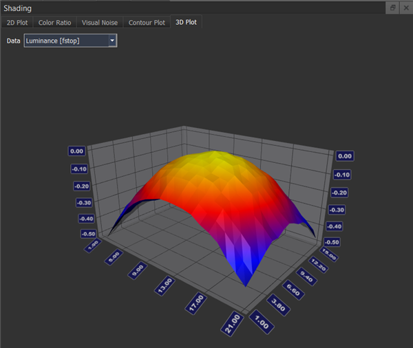
The “3D Plot” shows the uniformity over the columns and rows of the ROIs as an interpolated color-coded 3D rendering. The scaling of the color coding can be changed in the “Visualization” settings. By holding down the right mouse button and dragging, you can change the perspective of the plot.
Numerical Results
Shading(f-stop): The maximum shading of luminance Y in f-stops.
Shading(%): The maximum shading of luminance Y visible in the image. This value is calculated with Y as a weighted sum of R, G, and B, which is not affected by the linearization.
CIE ∆L: The absolute average shading of luminance based on CIE ∆L.
CIE ∆Eab: CIE ∆Eab expresses the maximum color shading over the image field as the maximum color difference. It conforms to the Chrominance Non-Uniformity defined in ISO 17957:2015 and the Color Uniformity defined in IEEE P1858 Standard for Camera Phone Image Quality (CPIQ). In contrast to the ∆E calculation used for color reproduction, the calculation of ∆Eab is done without luminance L*. So you get information only about differences in colors, without luminance.
CIE ∆C: CIE ∆C is the maximum color shading related to a defined reference value.
R/G(DV): The average green and red channel ratio in digital values.
B/G(DV): The average ratio of a blue and green channel in digital values.
Delta SNR(dB): The maximum Delta of SNR over all ROIs.
Delta VN Set1-3: The maximum Delta of Visual Noise overall ROIs.
Distortion
Image distortion occurs when the straight lines of a scene appear to be deformed or curved unnaturally in an image. There are three types of lens distortion called barrel, pincushion, and waveform, also known as mustache distortion. It is important to know that distortion occurs differently depending on the lens system and whether the lens can or cannot be removed from the camera. The iQ-Analyzer-X uses test patterns, crosses, or points distributed over the entire image field with a known position. The center location of the crosses or points is detected with sub-pixel precision and referred to as the target position.
Graphical Results
Distortion
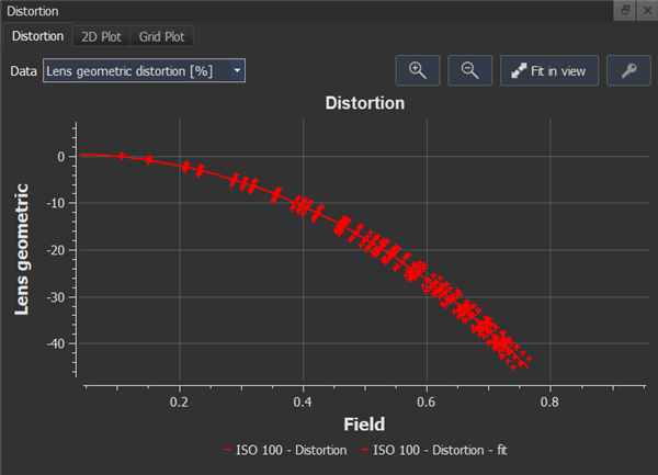
The “Distortion” plot shows the Lens Geometric Distortion or Chromatic Aberration over the image field. The image field is the radial distance from the image center to the image corner, mapped from zero to one. A detected point in the corner has a value near one and a detected point in the center near zero.
2D Plot
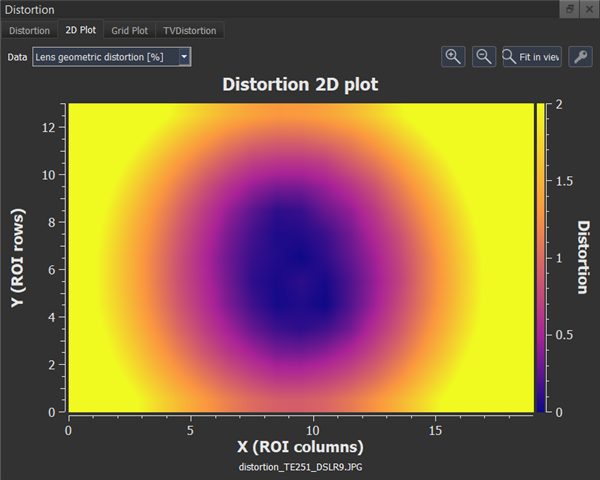
The “2D plot” shows the Lens Geometric Distortion or Chromatic Aberration over the rows and columns of the detected grid, typically crosses, points, or black and white markers. The color shows the intensity of the Lens Geometric Distortion or Chromatic Aberration in percent. The color map is shown on the right side of the graph; adjust its limits in the settings under visualization.
Grid plot
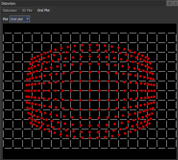
The “Grid plot” shows the detected ROIs as red spheres versus a grid with the expected locations. The farther the sphere is off from its location in the grid, the higher the distortion.
Quiver plot
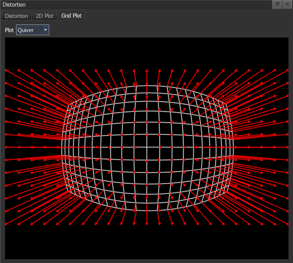
The “Quiver” plot shows the distortion by a vector pointing to its direction.
Note: In the “Quiver” plots, the length of the arrows does not reflect absolute and comparable values but only the directions. The arrows are scaled so that they can be seen clearly, and they only reflect the relative distortion or CA values to each other.
Quiver CA plot
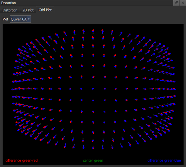
The “Quiver CA” plot also shows vectors for the chromatic aberration of red and blue.
TV Distortion
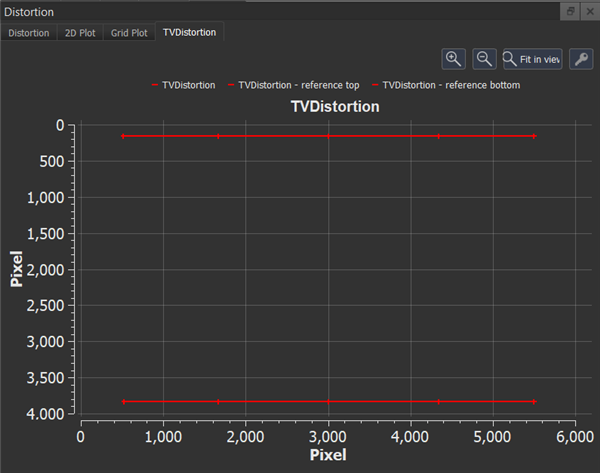
The “TV Distortion” plot shows the pixel coordinates of the markers used to calculate the TV distortion.
Numerical Results
Line Geometric Distortion (LGD) according to ISO 17850
LGD is defined as below.
Line GD Horizontal:
LineGD h: Line Geometric Distortion in the horizontal direction
A: Maximum height of the line grid pattern of the output image in pixels
B: Minimum height of the line grid pattern of the output image in pixels
V: Number of pixels of the short side of the frame of the output image
i: Suffix presenting each picture height
Line GD Vertical:
LineGD v: Line Geometric Distortion in the vertical direction
α: Maximum width of the line grid pattern of the output image in pixels
β: Minimum width of the line grid pattern of the output image in pixels
V: Number of pixels of the short side of the frame of the output image
i: Suffix presenting each picture width
Line GD Total:
TV Distortion
The results of distortion calculation are shown as EBU-TV-Distortion and SMIA-TV-Distortion (SMIA = Standard Mobile Imaging Architecture). The SMIA definition has been widely adopted in the mobile imaging industry.
EBU(%): EBU TV distortion is the change of image height from the center to the edge of the image, expressed as a percentage of the actual height in the center.
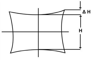
SMIA(%): SMIA defines distortion as the ratio of the absolute image height at the edges of the image to the image height in the center.
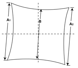
EBU-TV-Distortion and SMIA-TV-Distortion are similar measurements and contain the same information. SMIA-TV-Distortion is always double the EBU-TV-Distortion.
Lens Geometric Distortion (LGD) according to IEEE P1858, similar to Local Geometric Distortion in ISO 17850
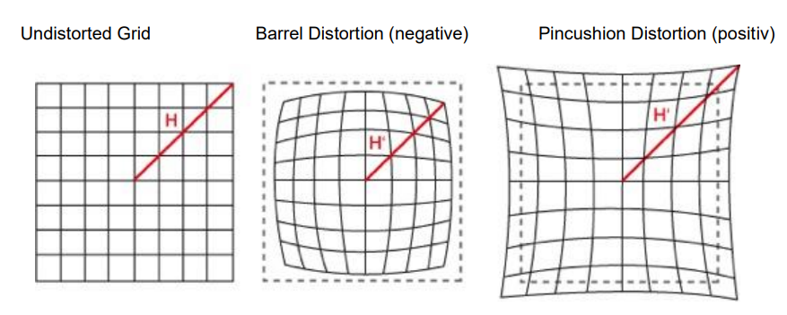
LGD is defined as:
H' = Actual dot distance from the center of the image
H = Expected dot position
The geometric distortion for a grid position is the delta between the radial distance of the actual grid position H' and the radial distance to the ideal grid position H, divided by the ideal grid position H.
For each detected point in the grid, the LGD is calculated.
H'< H indicates negative distortion → barrel distortion.
H'> H indicates positive distortion → pincushion distortion.
LGD mean: The average geometric lens distortion of all grid positions.
LGD worst: The maximum LGD of all grid positions.
LGD worst(fit): The worst LGD value fitted to a polynomial, which degree is defined in the “Distortion” settings.
Chromatic Aberration (CA)
CA G/R mean: The average pixel distance between the green and red channels.
CA G/R max: The mean value of the ten largest distances between green and red.
CA G/B mean: The average pixel distance between the green and blue channels.
CA G/B max: The mean value of the ten largest distances between green and blue.
LCD G/R [pix]: Lateral Chromatic Displacement in pixels between the green and red channel according to CPIQ. The distance between green and red channel is calculated based on polar coordinates. For the LCD G/R the maximum values for green and red channel are used.
LCD G/R [%]: Lateral Chromatic Displacement in percent of the picture height between the green and red channel according to CPIQ. The LCD G/R in pixels is set in relation to the image height in pixels.
LCD G/B [pix]: Lateral Chromatic Displacement in pixels between the green and red channel according to CPIQ. The distance between green and blue channel is calculated based on polar coordinates. For the LCD G/R the maximum values for green and red channel are used.
LCD G/B [%]: Lateral Chromatic Displacement in percent of the picture height between the green and red channel according to CPIQ. The LCD G/B in pixels is set in relation to the image height in pixels.
—-
Longitudinal Chromatic Aberration (LCA)
LCA Total: Mean value of the longitudinal chromatic aberration.
LCA Horizontal: Longitudinal chromatic aberration in the horizontal direction measured on the center cross (horizontal line of the cross).
LCA Vertical: Longitudinal chromatic aberration in the vertical direction measured on the center cross (the vertical line of the cross).
Export Results
The results can be exported as a *.xml or *.pdf file from the “File” menu. In the *.xml file, all numerical results will be saved. You can use this file to create your custom report. The *.pdf export provides basic layout adjustments and an option for which measurements will be included.
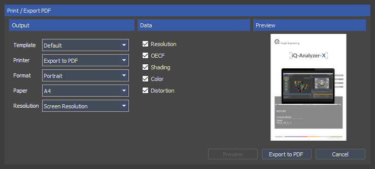
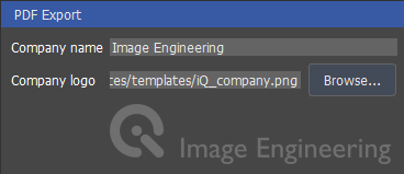
In the “General” tab under “Configuration” a custom logo and your company name can be inserted to appear in the .pdf report.
In the “PDF Settings” tab under “Configuration” you can define, which metadata and settings are added to the report.

The generated report shows only the image(s), which are selected in the “Input dock”.
Configure
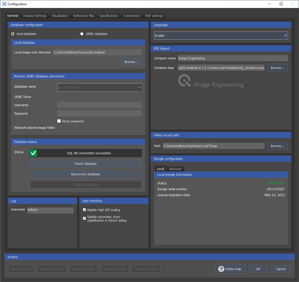
General
Database configuration
Select the database where you want to store your data. You can work with a local or remote database and switch between them.
Local image root directory
This is the path where the images of your analysis are stored. You can choose a different folder by clicking “Browse…”.
Remote ODBC database connection
Provide the required data to connect to your remote ODBC database.
Database status
You can check the database status and reconnect it in case of any changes.
User Interface
“Disable automatic chart classification in import dialog”- By activating this checkbox, you can prevent iQ-Analyzer-X from trying to find a suitable chart layout. It makes sense to activate this checkbox if you are working with custom charts that are not known to iQ-Analyzer, or if the recognition leads to a chart that has to be specified by the user anyway, such as the TE269V2.
Language
Set your preferred language here.
PDF Export
Set your company name and logo and include them in your exported *.pdf reports.
Log
Set the username that will appear in the log.
Dongle Configuration
Displays information about the local or network dongle currently in use.
Analysis Settings
In the “Analysis Settings” menu, you can define the measurements and parameters for your image analysis. The settings can be saved to the database to make a repeating application easy. To apply the settings to your analysis, you need to select them in advance in the input dock.
Note that you can also update your settings with new values. When you do this, the “ID” number of your settings will change. The old settings are still in the database under the old ID in case they were used for a previous analysis. This is important to know if you work with CLI scripts. You may need to change the IDs in your script as well.
Analysis tab

In this tab, you can define the measurements carried out when you start an analysis. Please note that some measurements might not be available, depending on your chart. To apply your settings you need to save them first. The right column only applies to UTT charts.
Resolution tab
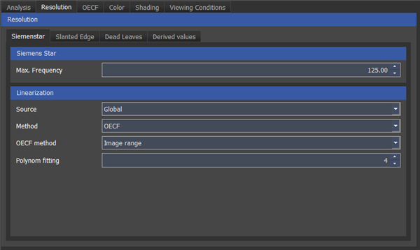
Three different methods for measuring resolution can be applied with iQ-Analyzer-X - Siemens star, slanted edge, and dead leaves. All of the methods have the same options for linearization.
Source: Depending on your chart, you can choose between local, global, and no linearization.
- Local: The gray patches close to your measurement target are used. Example: In the TE268 (25 Siemens stars), each star is linearized with the local gray patches around each star.
- Global: A single set of gray patches is used for linearization. For example, in a TE42V2 or the TE268 target, the OECF patches in the center are used.
Method:
- Profile: If you choose “Profile,” the image will be linearized based on the color space of your image (e.g., sRGB).
- The “OECF” setting takes the measured OECF into account.
OECF method:
- Data range: The entire data range is used for the calculation (e.g., 0…255 for 8bit images)
- Image range: The gray patches' minimum and maximum digital value is used.
- Normalized image range: If black and white reference patches are available, these are used to normalize the modulation.
- MTF: An older approach where the black value is subtracted from the image to achieve a de-facto normalization.
See this paper for details: https://www.image-engineering.de/library/conference-papers/862-linearization-and-normalization-in-spatial-frequency-response-measurement
Polynomial fitting: Defines the degree of the polynomial fitting curve for the OECF.
Siemens Star
Maximum frequency: You can choose what frequency iQ-Analyzer-X calculates the modulation. The value is provided as a percentage of the Nyquist frequency. So if the Nyquist frequency is 1000 LP/PH and you set the maximum frequency to 125%, iQ-Analyzer-X will analyze the radii that equal frequencies lower than 1250 LP/PH. The edge of the Siemens star defines the lower frequency limit.
Slanted Edge
- Polynomial fitting: The degree of polynomial fit for linearization can be adjusted.
- Max. Frequency: See Siemens star.
- Edge Profile Source: You can choose between original or linearized data.
- Color Channel: You can choose if the SFR for RGBY or only Y should be measured.
Dead Leaves
Analysis Method: You can choose between three different calculation methods for Dead Leaves - Core, Direct, and Cross. Cross is the recommended method as it is robust against noise's impact. Please refer to this paper on our website for more detailed information about the differences.
Derived values
Here you can specify the parameters you want to show in the results. These are values that are calculated based on an SFR.
OECF tab
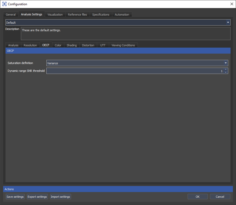
Saturation definition
Variance: Saturation calculation is based on the variance of the DVs.
Dynamic range SNR threshold
The dynamic range is the difference between the illumination needed to reach saturation and the minimum illumination defined by a specified SNR value. The standard value for ISO 15739 is SNR = 1. This value may lead to problems due to signal processing and noise reduction, as an SNR of 1 is never reached, and thus, the threshold might be increased. We have good experience using a threshold of three, and a threshold change should be reported if deviating from the ISO standard.
Color tab
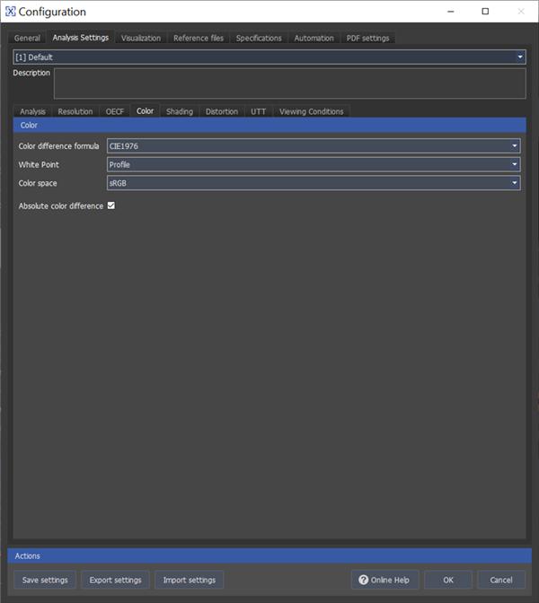
Color difference formula
The iQ-Analyzer-X calculates Delta E from two Lab data sets, the reference, and the image sample set. You can choose between CIE1976, CIE1994, CIE2000 and CIE2000 SL1 formula for calculating Delta E, with the most common being CIE1976. A more detailed description of the details is in the “Results” section.
White Point
Currently, the only option is to take the white point from the image profile.
Color space
If the test image contains a color profile, the profile is automatically applied, otherwise the color space selected here is used.
Absolute color difference
Activate this check box if you want to get results with absolute values. Absolute values only represent the number of color differences but not the direction.
Shading tab
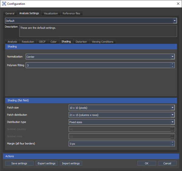
Normalization
“Brightest” sets the coordinates with the maximum luminance as a reference for normalization (reference = max. luminance = 0). This option makes sense if your brightest patch shows an offset to the image center due to misalignment of the lens to the sensor. “Center” applies to the center of the image for normalization (reference = center = 0).
Polynom fitting
“Polynom fitting” defines the polynomial degree that is fitted to the data.
Patch Size
“Patch Size” defines the size of the shading ROIs in pixels.
Patch distribution
“Patch distribution” defines the number of columns and rows of the shading measurements.
Distribution type
“Fixed Sizes” takes the “Patch Size” and the “Patch Distribution” value to generate the grid with the shading ROIs. “Seamless” creates a grid that leaves no empty spaces between the shading ROIs.
- “Number columns” defines the number of columns of the seamless grid.
- “Number rows” defines the number of rows of the seamless grid.
Margin (all four borders)
This value sets the size of a margin in pixels around the test image. Setting a margin makes sense if your image contains regions at the edge which you do not want to include in the shading measurement.
Note: As an ROI in the image center is required for shading measurements, only odd numbers are available for the rows and columns.
Distortion tab
In “Polynom fitting,” you can define the degree of the polynomial of the fitting algorithm for distortion calculation.
Viewing conditions tab
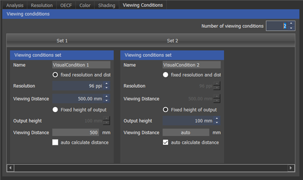
As the visual perception of noise depends on the viewing conditions, they need to be specified for the measurement of Visual Noise. You can either select “Fixed resolution and distance” or “Fixed height of output” for each condition.
Visualization
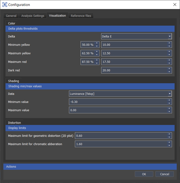
In this tab, you can specify the color coding of the scaling bar in some of the result plots.
Color - Delta plots thresholds
You can scale the color mapping for the graphical results for delta E, L, C, H, and VN. Either enter a relative limit in percent from the maximum (dark red) or an absolute value.
- “Minimum Yellow” defines the lowest value that is still yellow.
- “Maximum Yellow” defines the highest value that is still yellow.
- “Maximum Red” defines the highest value that is still red.
- “Dark Red” defines the value from which the plot will be dark red.
Shading - Shading min/max values
Only the “Contour Plot” and the “3D Plot” are affected by these settings.
- “Data” defines the parameter for which you can change the minimum and maximum values.
- The “Minimum Value” is plotted in blue.
- The “Maximum Value” is plotted in yellow.
The plots update as soon as the minimum or maximum value is changed.
Distortion - Display limits
- “Maximum limit for geometric distortion (2D plot)” defines the maximum distortion value for the color map in the 2D plot.
- “Maximum limit for chromatic aberration” defines the maximum value of chromatic aberration for the color map in the 2D plot.
Reference Files
A reference file (*.ref,*.xlsx) or measurement data (.pdf) will be provided for most image engineering charts on our download server . It contains your chart's luminance, density and/or color measurements. In some cases, you need to create the reference file manually from the measurement data. Please refer to “Creating and Editing Reference Files” for instructions.
Note, that not all charts need a reference file to be analyzed properly. In some cases, the software already knows what to expect, and the measurement data in your acceptance protocol is only used for quality control. Also, some metrics as distortion or shading do not require reference data.
UTT users only: The UTT reference files are in *.xlsx format. Note, that an MS Excel Version needs to be installed for UTT reference files on your computer to import the file properly into the database!
Here is an overview about the availability of individual *.ref files or measurement data for the test charts currently supported by iQ-Analyzer-X.
| Chart | before 2024 | from 2024 on | comment |
|---|---|---|---|
| TE165 | Not Applicable | Not Applicable | - |
| TE188 | *.pdf measurement data | Individual *.ref file provided | Additional *.ref file for placing test chart in scenes |
| TE230 | *.pdf measurement data | Individual *.ref file provided if ordered | Additional *.ref file for placing test chart in scenes |
| TE240 | Default Reference Data only | Default Reference Data only | - |
| TE251 | Not Applicable | Not Applicable | - |
| TE253 | Not Applicable | Not Applicable | - |
| TE255/Flatfield | Not Applicable | Not Applicable | |
| TE258 | *.txt file xxx | Individual *.ref file provided | - |
| TE259 | *.pdf measurement data | Individual *.ref file provided | - |
| TE260 | Not Applicable | Not Applicable | - |
| TE261 | Not Applicable | Not Applicable | - |
| TE262 - UTT | Individual *.xlsx file provided | Individual *.xlsx file provided | - |
| TE264 | *.pdf measurement data | Individual *.ref file provided | - |
| TE268 | Not Applicable | Not Applicable | - |
| TE269 | *.pdf measurement data | Individual *.ref file provided | - |
| TE270 | *.pdf measurement data | Individual *.ref file provided | - |
| TE275 | *.pdf measurement data | Individual *.ref file provided | - |
| TE276 | *.pdf measurement data | Individual *.ref file provided | - |
| TE283C | *.pdf measurement data | Individual *.ref file provided | - |
| TE284 | *.pdf measurement data | *.pdf measurement data | - |
| TE295 | *.pdf measurement data | Individual *.ref file provided | Individual *.ref file for each head and siemens star |
| TE296 | Not Applicable | Individual *.ref file provided | - |
| All TE42 | Individual *.ref file provided | Individual *.ref file provided | - |
| Lenstester | Default Reference Data only | Default Reference Data only |
Import the reference file and add it to the database in the “Reference Files” tab in the “Configuration” dialog. If you do not have a reference file for some reason, you can also work with the default reference data. However, an individual reference file is more accurate as it compensates for variance in chart production.
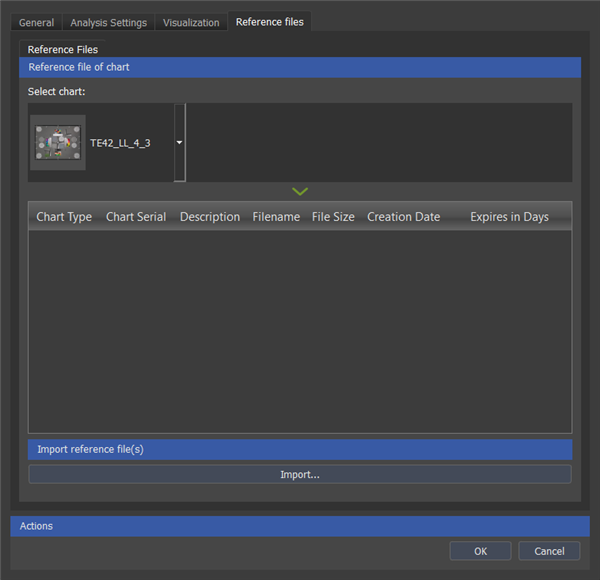
Click on “Import” and select the reference file you want to import. In the upcoming dialog, you can see information about the file and edit the serial number and description by double-clicking on it.
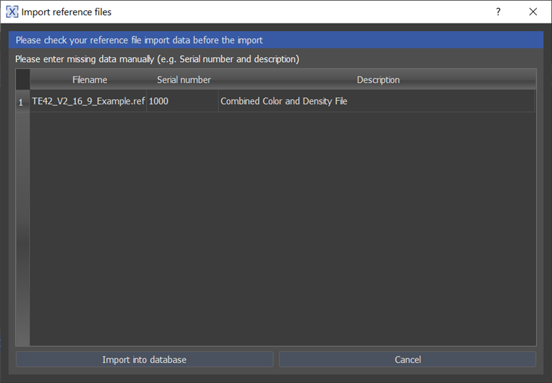
A successful import shows the message below.

To review the reference files which have already been imported, select your chart in the dropdown menu. Note that you can still edit the serial number and the description of the reference file by double-clicking on the desired field. This feature makes assigning the reference to an image in the import dialog easier.
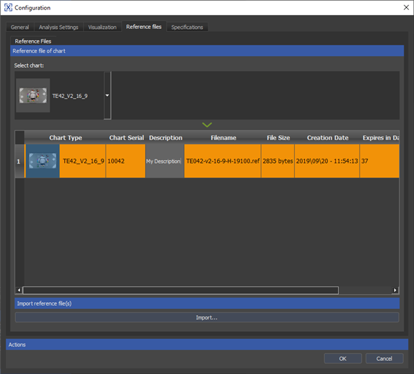
Right-click the entry and choose “Remove reference file from database” to remove it.
Reference files are only valid for a certain period of time, depending on the material of the test chart. In most cases, the service life is stated in the data sheet. You can see the expiration date of the reference data when you select it in the import dialog or in the “Reference files” tab under “Configure”.

The “valid period” is derived from the “Creation Date” and “Valid For” values stated in the *.ref file.
If your *.ref file is newer than the test image, you get a warning, as the reference data is expected to be created before the first test images.
After a successful import, you can allocate the reference file to your chart before your analysis in the "Import" dialog.
Creating and Editing Reference Files
Sometimes, you need to create the reference files yourself or update them with your measurements.
Currently, two file formats for reference files can be imported into iQ-Analyzer-X, Excel (.xlsx) and the proprietary format (.ref). The Excel format is exclusively for UTT, and .ref is for all other charts. If one of these files is provided with your chart, you can import them into the database without making any changes. Some of our charts are delivered with a .pdf acceptance protocol containing all measurements. In that case, you need to create the .ref file manually. Note that the .ref file is in YAML format, a standard markup language.
To create or update a reference file, you first need to copy the current example reference file from the reference folder.
C:\Program Files\Image Engineering\iQ-Analyzer-X 1.X.X\resources\references
Open the copied file and update it with the measurements of your chart. Depending on your chart, the reference file might contain color, density, luminance values, or multiple metrics. Note that it is crucial to keep the file's formatting as it is; otherwise, the software might not be able to read it. The best way to do that is to select the value you want to change and then type in the new value.
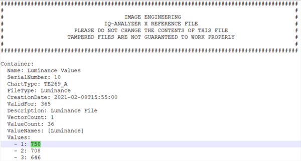
In addition to the color, density, or luminance values, you can edit the following entries in the file header:
Name: The name of the container. A reference file can contain multiple containers, which include all required information for a specific metric, such as OECF, Resolution, etc.
SerialNumber: Provide the serial of your chart to make it easier to find the relevant reference file during image import. After importing, you can still change the serial number in the “Reference Files” tab.
FileType: FileType can be Color, Density, or Luminance. In most cases, you do not need to change it; however, you may want to work with luminance instead of density or vice versa. In this case, change the value accordingly.
CreationDate: The creation date of this reference file. Be sure to keep the formatting.
ValidFor: The validity of this reference file in days. “CreationDate” and “ValidFor” provide the required information for the iQ-Analyzer-X to calculate the expiration date of your reference data.
Description: Add a description. It makes it easier to find the relevant reference file during image import. After importing, you can still change the description in the “Reference Files” tab.
All other entries in the header of the file must not be changed!
Reference files for OECF charts can contain either densities or luminance. This is an example of a density .ref file for a TE269 V2.
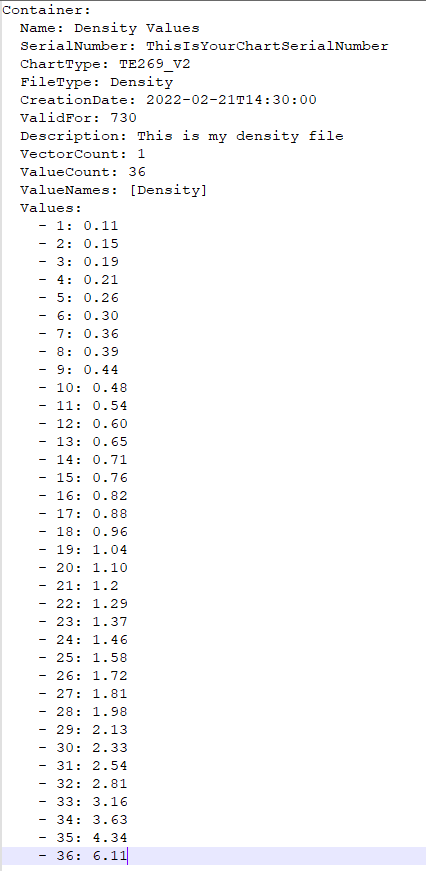
This is an example of a luminance reference file for a TE269 V3, which you can find in the folder “references”.
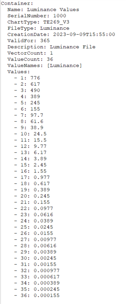
After editing your reference file, save and import it into the database, as explained above.
Accuracy of reference data
Our densitometer uses directed light. Changing the illumination geometry to diffuse light can lead to a different contrast of the photographic film. This effect is known as the Callier effect. Please note, not every film material is affected in the same way. For the most accurate measurements, we recommend determining the luminance data with an appropriate luminance meter. Using the luminance reference data, if determined with light source of test setup, will prevent potential inaccuracy based on density data.
On high dynamic range OECF charts, the dark patches do have a very low intensity and are difficult to measure, especially when you do not have a powerful light source. As a workaround, you can also derive the luminances from the brightest patch and the densities from the acceptance protocol. Note, that transmissive charts also reflect into the light source and thus have an effect on the intensity. By measuring the brightest patch, this effect is taken into account.
More information about reference data accuracy you can find in this document.
Video File and Webcam Video Analysis
To use this feature, your operating system needs to know the video codec to open video files and import frames from it. It might be necessary that you install the required codec first before using this function. If you are having trouble importing a video, please follow this link.
The following options are available to analyze videos.
- Record a video from a connected camera known by the operating system or the integrated webcam.
- Record a video from a live stream with a known URI (Uniform Resource Identifier)
- Open a video file, which codec is known by the operating system
- Capture videos from a server with the iQ-Analyzer-X Capture Server tool.
From this video files you can either take specific frames and analyze them as explained under "Analyze Images" , or you can import specific ranges of the video file and measure specific metrics over time.
It's also possible to measure MTF, Color and other metrics live from a connected camera known by the operating system or the integrated webcam.
Click on “New Analysis” and then on the “Import Video” button.

This shows up the “Import Video” dialog.
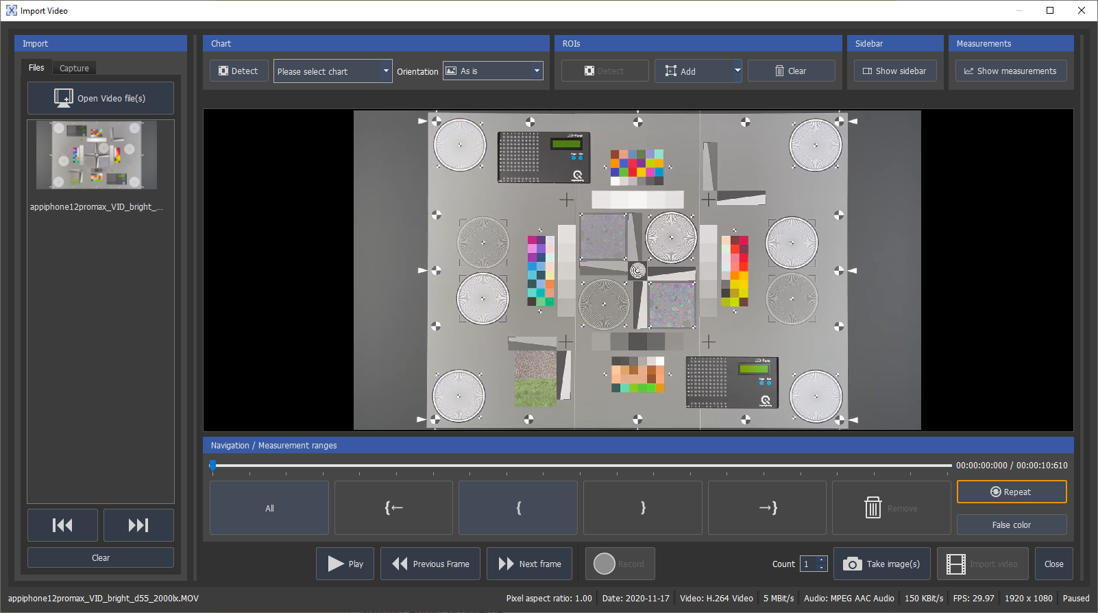
Import Video from Webcam
Open the “Import Video” dialog and select the “Capture” tab. All available cameras will be shown under this tab. Select the camera you want to take images from. Select your desired video format in the dropdown menu “Available Formats”. You can either record a video or you can also capture images from the stream with “Take image(s)”. The number of images you take is set with “Count”.
The recorded videos are stored under the path you defined in the “General” tab in the configuration dialog. Default is /Appdata/Local/Temp.

The recorded videos show up under the “Files” tab.
Import Video from a video livestream
In the “Import Video” dialog select the “Files” tab. Click on “Open Video Stream” and enter the URI of the livestream you want to capture. The stream address shows up in the file list. You can either record a video which also is added to the file list, or you can also capture images from the stream with “Take image(s)”. The number of images you take is set with “Count”.

Mark the recorded video in the file list to do further analysis.
Analyze single Images/Frames from Video
You can capture images of all the videos shown in the viewer. It doesn't matter, if it is live or an already existing file.

For example, if you open a video file, move to a frame you would like to import with the slider below the viewer and click “Take image(s)”. With “Count” you can define the number of images you take from that position on forward. These images immediately appear in the “Import” dialog. You can repeat taking images from different positions in the video. In case of a livestream the slider is disabled and the images are captured at the time you press “Take image(s)”. When you have taken all the desired images, close the “Import Video” dialog. The “Import dialog” is still open and shows all the selected frames.
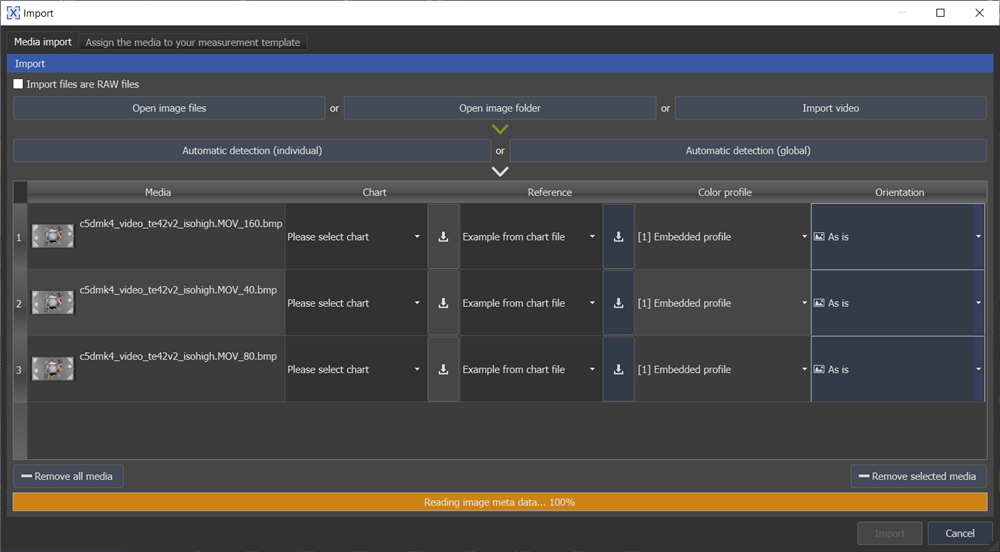
Assign a “Chart”, a “Reference”, a “Color Profile” and change the orientation of the images if necessary. With the “arrow down” button, you can assign your selection to all the images. Click on “Import”. Now the images are displayed in the “Input dock” and are ready for analysis.
Tip: Add a ROI and assign a measurement to find frames with specific best or worst results.The procedure is explained in the following section.
Allocate measurements to a target in a recorded video or a live stream from a connected camera
You can add ROIs and assign measurements to Videos. Once you have done this, a plot with the measurement will appear on the right. If you now move the slider, the plot will draw the measurement depending on the position of the slider. This is very useful if, for example, you want to import only the frames with the best or worst results, or at all. Available measurements are RGB, LCH, Visual Noise, Slanted Edge MTF and Standard Deviation. The measurements can also be performed on a video live stream or a stream from a connected camera. For example, it is possible to stream a livestream, from an IP camera. To do this, the URI (Uniform Resource Identifier) must be known and the device must be connected to the same network.
Add your own ROI with “Add”. “Detect” performs an automatic detection of ROIs on the video file. The detection only works when a chart layout is defined and adds ROIs only for the targets which support live measurement. With “Add” you can add your own ROI. The size and position of the ROIs can be changed in the viewer. To edit a ROI, open its context menu with a right-click on the ROI and select “Rename” or “Delete”. If you have multiple videos in the “Import” section, the ROIs are applied to all of them.

You can also import previous ROIs in .xml format or export your current ROIs.
Set the desired measurement for the ROI by right-clicking on it and selecting the metric. The following screenshot shows the currently available metrics.
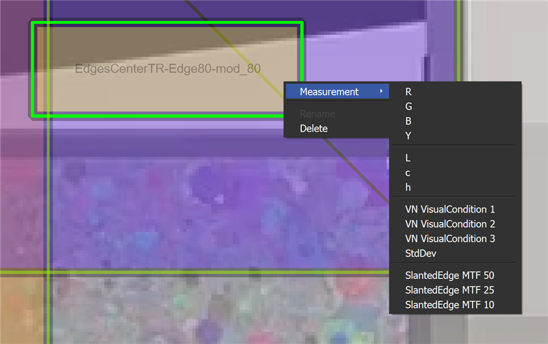
The measurements show up on the right side of the dialog in a plot. If you now move the video slider from one frame to another, the measurement of the frames will be added to the plot. In case of a live stream measurement, the feature will plot the result of the current frame.
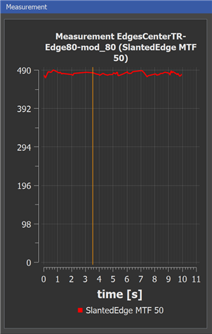
Tip: Use this function, for example, to adjust the manual focus of a DUT.
Analyze Video Files over time
This feature only works with video files instead of single images, and the results show the measurements over time. Note, to get results it is required to define a ROI and assign a metric to it as described in the previous section.
Open a Video File in the “Import Video” dialog or record a video from a connected camera or a livestream. If applicable, define the chart layout either with auto-detection or manually using the dropdown menu. The classification will be kept the same for multiple videos, if you activate the paper clip button. You can also autodetect the ROIs by pressing “Detect” in the ROIs section. The metrics you want to measure need to be assigned manually per ROI by right-click on the ROI.

In the navigation section, you can now select a part or several parts of the video, which you want to import. If you want to import the entire video, click on “All”(1) and then “Import Video”. To import a specific range of the video, move the video slider(7) to the desired start position and click “Set in Point”(3). Now move the slider to the last frame you want to import and click “Set out Point”(4). The selected range is now marked blue on the slider scale. Add another range by repeating the process. You can skip through the in and out points with button(2) and (5). To delete a range, place the slider over the marked area and click on the “Remove”(6) button. If you are done, click “Import Video” and close the “Import video” dialog.
Assign the “chart”, “reference”, “color profile” and “orientation” information to the video.
Note, that the dialog only shows one file, even if you have selected multiple parts of the video.
Analysis and Results over time
The video shows up in the “Input dock”. Choose the “Settings”, leave “Detection” on “Automatic Mode” and start a new analysis. The results, measurement over time, appear in one tab.
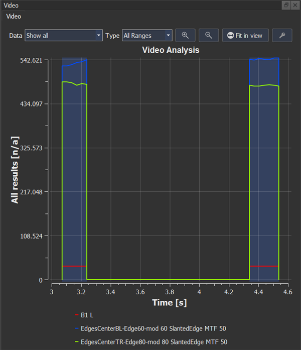
Select the measurement you want to see under “data”. Under “Type” you can select the range which you defined during video import. The selected view will be the one visible in the .pdf report.
The imported video with its selected ranges is shown in the “Media Display”.
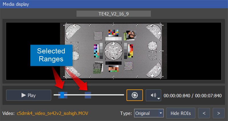
VCX-WebCam Analysis
Click on “New Analysis” and open the “Import” dialog. In the “Import” dialog, click on “Import video” to open the “Import video” dialog. Open the desired video file(s). The videos are shown in the “Import” section. Click on the video you want to process. The selected video will be highlighted. Note, that you can also capture videos remotely from your DUT using the "iQ-Analyzer-X Capture Server tool".

You can automatically assign the chart with “classify” or choose a chart in the “Please select chart” dropdown menu.
The classification will be kept the same for multiple videos, if you activate the paper clip button.

If the chart type is set properly, continue to the VCX metric you want to measure. Auto Exposure and Auto White Balance are available in the VCX dropdown menu. You can change the rotation of the image if necessary. If everything is ok, detect the ROIs by clicking “Detect”.
The detected ROIS are shown in the video viewer. If you have multiple videos in the “Import” section, the ROIs are applied to all of them.
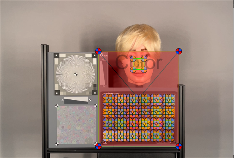
To import or export ROIs click on the small white arrow next to “Add”.

You can also load the default ROIs by clicking the white arrow next to the “Detect” button.
If you need to edit the ROIs for some reason, open the sidebar, to have more options. To do so, click the “Visibility” tab and click on “Show sidebar”. The same options are available as explained in chapter ROI Detection. Note, that there are some useful tips to edit the ROIs in this chapter.
When all ROIs are properly adjusted, you can start to assign measurements to them. Currently, the required measurements are automatically added to the corresponding ROIs, by selecting “Auto White Balance” or “Auto Exposure”, but they show no plots. As a workaround, you can add the plots for L* an C*. Right-Click on the ROI and activate L* and C*.
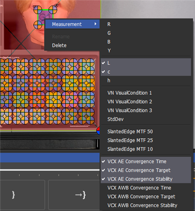
The selected measurement show up immediately under the “Measurements” tab.
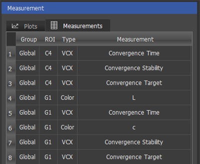
Play the video to see a live measurement of the metrics under the “Plots” tab.
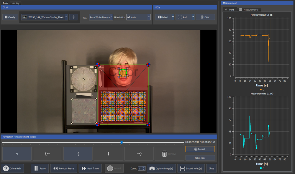
Click on “Import video(s)” to add the video to the “Import” dialog and close the window.
At last, assign the reference file and the color profile to the video and click on “Import”.
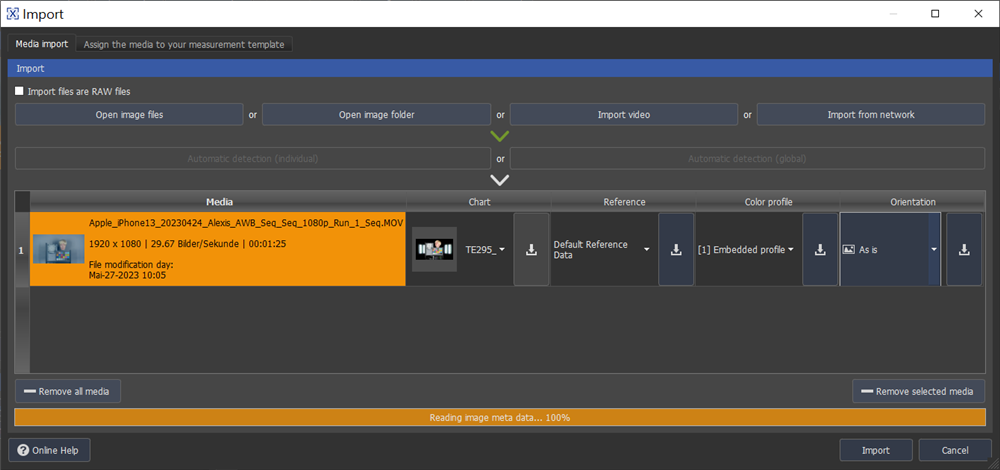
The video shows up in the “Input” section. You can now start the analysis by clicking “Start New Analysis”.
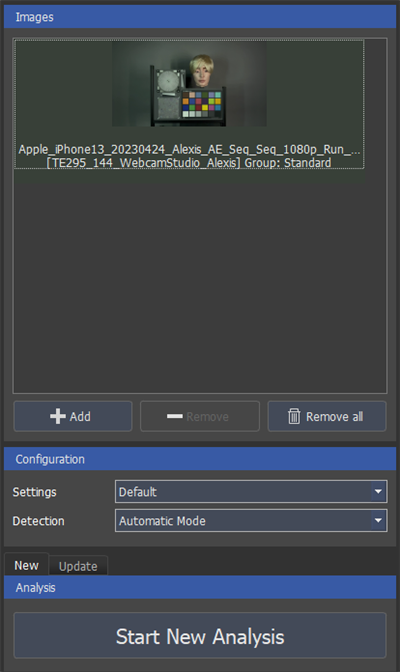
VCX-WebCam Results
Graphical results
Currently, for VCX-WebCam only numerical results are available. However, if you assigned additional measurements to the ROIs manually, the plot of this metrics shows up.
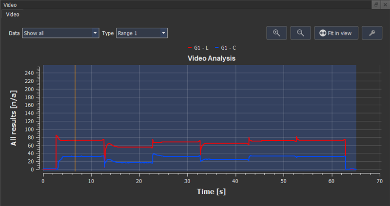
Numerical results
The numerical results of AWB convergence time, AWB convergence stability and AWB convergence target for each illumination step are shown in a result table.
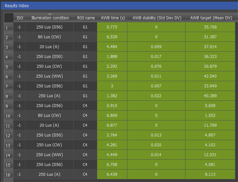
The numerical results of AE convergence time, AE convergence stability and AE convergence target for each illumination step are shown in a result table.
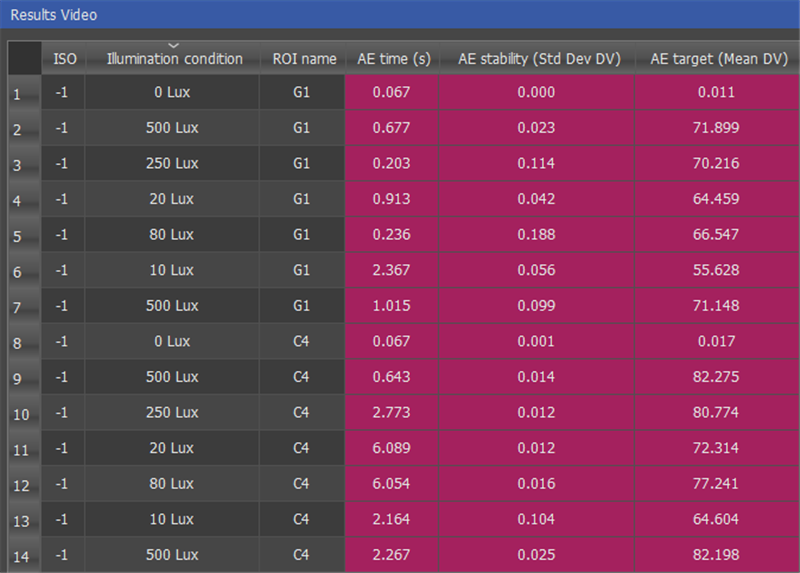
For a detailed description of the numerical results, please refer to the actual VCX-WebCam paper.
Import Images from a remote Webcam using the iQ-Analyzer-X Capture Server tool
In the case you want to capture images from a webcam which is integrated in a laptop, it can be complicated to control the capture process and alignment as the test device is mounted in front of the test chart. You can use the iQ-Analyzer-X Capture Server tool to make things easier. The tool allows connecting to a network server located on the test device and capture videos or frames from its webcam. The two devices just need to be connected to the same network.
Follow these steps to establish a connection.
First, install the iQ-Analyzer-X Capture Server tool on the device under test and run the software.
The installer, iQ-Analyzer-X_CaptureServer_setup.exe, is located in the folder C:\Program Files\Image Engineering\iQ-Analyzer-X 1.X.X\install.
After installation, run the software.
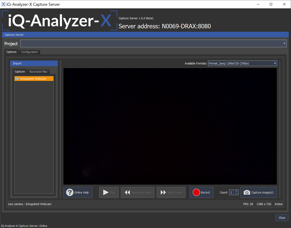
Click on the webcam under test to activate it. The webcam image appears in the viewer.
Then switch to the configuration tab to set up your capture server.

Network server
Host: Enter a name for the capture server
Port: Provide a port number
Active: Activate the switch to make the server visible for the remote client.
Server access authentication
Active: Activates the server access authentication. The server will request a username and password to establish connection.
Provide a username and password for the login from your client.
Local configuration
Provide a record path, where the captured videos will be stored, and a naming convention.
At last, add a project and enter a name in the project list.

Start iQ-Analyzer-X on your remote workstation. Click on “Remote” in the toolbar

Or click “Import from network” in the “Import” dialog.
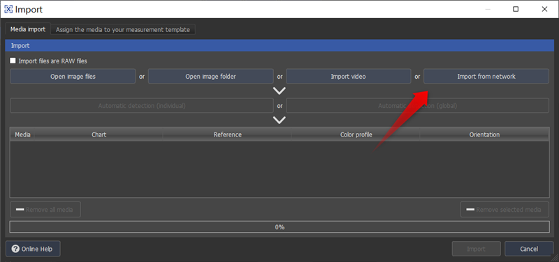
In any case, the “Network Capture Client” opens, but if you have chosen “Import from network”, you are able to add the images directly to the “Import” dialog.
If you have set the server “Online”, it will be listed in the “Selected Server” dropdown menu. Provide the username and password in the “Credentials” tab if you enabled the “server access authentication” on your capture server.
When your server is selected, the image of the webcam shows up in the view port.
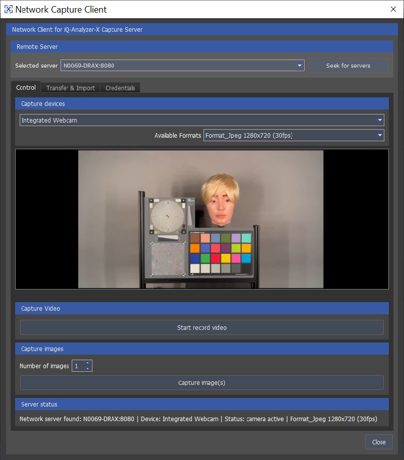
You can now capture a video or images. If you capture a video, the record duration shows up under the view port. Click on “stop record” to finish your capture.
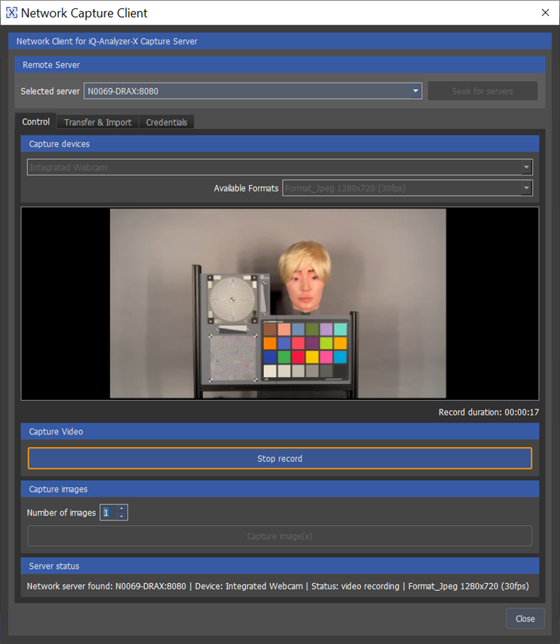
The captured videos are listed in the “Transfer&Import” tab and can be downloaded on the client from there.
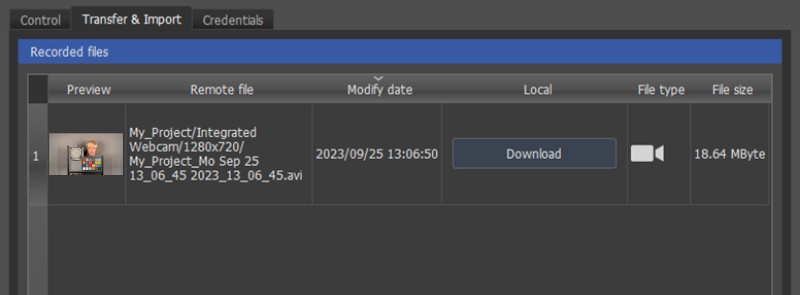
If you are experiencing any issues with the connection, please check your firewall settings or consult your IT.
UTT
The Cultural Heritage (CH) and the Pro version of iQ-Analyzer-X are designed to analyze the Universal Test Target (UTT - TE263) according to ISO 19264:2021, the Metamorfoze Guideline and color charts or targets. Further on, both versions of the Scan Reference Chart (TE263) are supported. It provides insight into the complete image quality of all high-end cameras and scanners.
The UTT target is available in the DIN sizes A4 to A0. The formats A3 to A0 consist of tiles with the same layout. A3 is one tile, A2 consists of two tiles, A1 of four tiles, and A0 of eight tiles. The A4 format has a slightly modified design, with only two gray scales and one set of color patches.
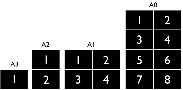
ROIs on the UTT
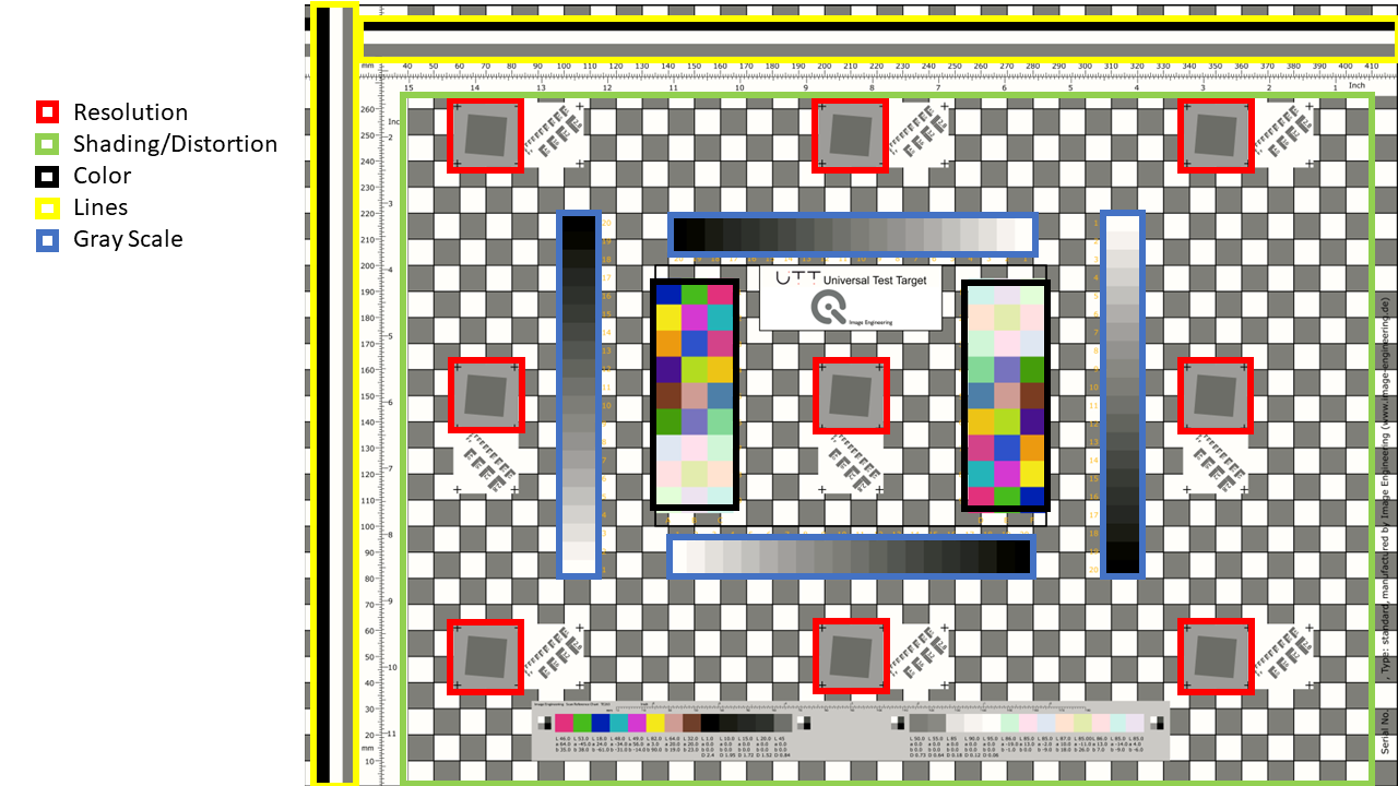
Lines: The yellow-marked areas are used to test for “dead lines” or banding that can occur during the scanning process.
Resolution: The nine red-marked areas with a slanted edge are used for resolution measurements.
Gray scales: The blue-marked areas are the four gray scales used for tonal reproduction, white balance, gain modulation, and noise measurement.
Color patches: The two black-marked areas are used for color measurements.
Shading + Distortion: All white and gray boxes in the green-marked background, which are fully visible and not hidden by a target, are considered for shading and distortion measurement. An example for a UTT DIN A4 is shown below. All the squares with red and blue frame are taken into account for the measurement.
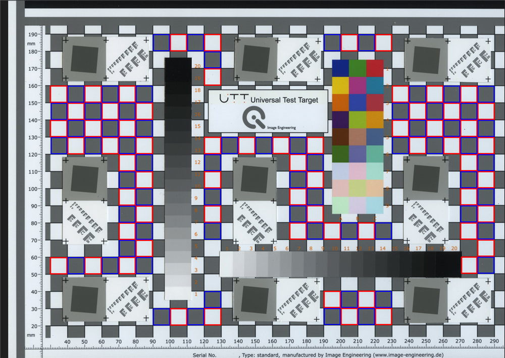
Specification
The specification files define limits for acceptable results. The definition of the levels is based on different applications such as Artwork, Unique Library, Non-Unique Library, and others. iQ-Analyzer-X already contains several specifications as Metamorfoze and ISO19264, in different variations. Metamorfoze, Metamorfoze light, and Metamorfoze extra light are the three levels defined in Metamorfoze Guideline. Metamorfoze is the strictest level, and Metamorfoze extra light has the highest tolerances. For details, please also refer to Metamorfoze Preservation Imaging Guideline. ISO19264:2017 is present in Levels A, B, or C. For more information about the differences, please refer to the ISO Standard.
Another option is to create a custom specification. To do so, copy the UTT Tolerance Sample from C:\Program Files\Image Engineering\iQ-Analyzer-X 1.X.X\resources\specifications to a local folder. Open the file as a .txt file in a standard editor.
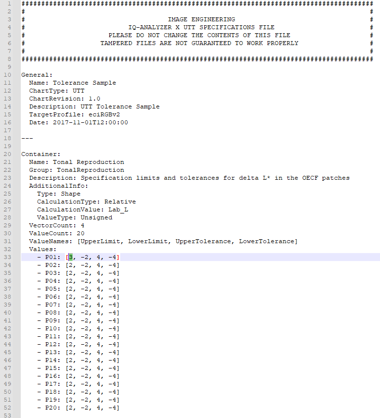
You can change the upper and lower limits and upper and lower tolerance for each measurement in the text file. It is important that you do not change the format and spacing in the file. The best practice is to select the limit/tolerance value you want to edit and type in the desired one. In the example above, we changed the upper limit in Tonal Reproduction for Delta L* in patch 01 from 2 to 3.
The tolerance values provide an additional classification. For example, your device under test can be outside the specification but still within the tolerance. The tolerance is displayed as a yellow area in the plots and results inside the tolerance.

Devices outside of the specification are marked yellow in the overview. If you do not want to add a tolerance, assign the same values as the upper and lower limit. Please also change the current name and the description under “General,” as this will be the information you see in the “Import” dialog. After editing the .txt file, save it and import it into the database in the “Specifications” tab under “Configure.” It is now available when you import your next UTT test image.
UTT Analysis
The UTT chart analysis works similarly to the image quality analysis described in the section Image Quality Analysis, but there are some differences. The reference file for your chart, which contains the measurement data, is provided in .xlsx format and will be automatically converted to a readable format for the software during import into the database. For this conversion, you need an installation of MS Excel or MS Office on the PC. Please contact our technical support team if you do not have the required software installed. The section "Reference Files" describes importing the reference file and changing the serial number and description. If you use an unmeasured chart, please select the “Default Reference Data” in the “UTT Import” dialog.
Note, that the reference file of your UTT is only valid for a certain period of time as the colors in the chart might degrade over time. You can find the expiration date of the reference data when you select it in the import dialog or in the “Reference files” tab under “Configure”.
In addition to the reference file of your chart, you need to select a specifications file that contains the specification you want to apply. The most common specifications are already provided. If you want to add a specification to the database, open the “Configure” dialog and select the “Specifications” tab. Click “Import” and select the desired specification file.
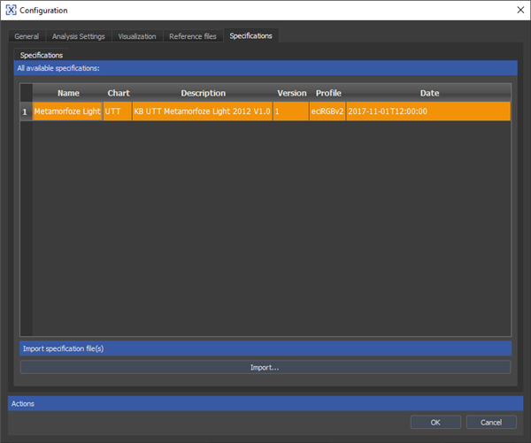
The specification file is now saved in the database and can be allocated in the “UTT Import” dialog.
“Note, that the UTT chart must be full frame, or the environment has to be nearly homogeneous. The most suitable is a homogeneous white, gray, or black background.”
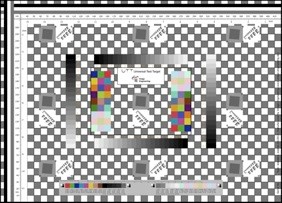
To start a UTT analysis, click “New UTT Analysis” and open the “UTT Import” dialog.

In the “UTT Import” dialog, you can define the chart, specification, reference, color profile, and image rotation. All the UTT settings are set automatically according to the specification you selected. If you select “Embedded Profile” and the color profile could not be found, the backup profile, which is defined in the settings, will be applied.
Note, that there is no autodetect for the chart layout, as the different UTT sizes, except A4, share the same layout. You need to assign the chart manually.
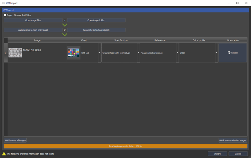
Click on the “Import” button. After the import, select the settings you want to apply, in case you created your own custom settings. If not, leave the dropdown on “Default”.

The “Detection” dropdown menu is on “Automatic mode” by default, which means that all the ROIs are assigned automatically. However, if you run into issues and a target is not detected properly, you can also select “Semiautomatic mode”. In this case the “Manual ROI Selection” dialog appears in which you can adjust the failed ROIs by yourself.

Please refer to chapter "ROI Detection" for more information about the “Manual ROI Selection” dialog.
Tip: If you always have the same setup, meaning that the chart is always in the same position in the image, you can use the template function in the “Manual ROI Selection” dialog. Here, you can save a ROI template and apply it to other images. Another option is to export your ROIs as .xml and apply them. They can also be applied in an automation process like Hotfolder or CLI to speed up the entire analysis process. Please refer to the chapter about automation for more information.
Click on “Start New Analysis”. All measurements are now being taken, and the results will be displayed afterwards.

UTT Results
After the UTT Analysis is finished, the results and an overview are provided. This overview contains a classification of the analyzed parameters, e.g., Tonal Reproduction, Noise, Color, Resolution, Shading, Distortion, and Lines, based on the applied specifications.
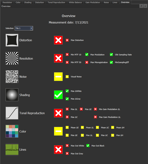

The result is outside the limits specified in the selected specification (Metamorfoze, ISO 19264, etc.).

The result is within the specified specification's limits (Metamorfoze, ISO Level A, etc.).

The result is outside of the specification but within the tolerance.
The numerical results are displayed in the UTT Results tab. Results within the specification are white, results outside the specification are red, and results in which the specification is not applied are grayed out.
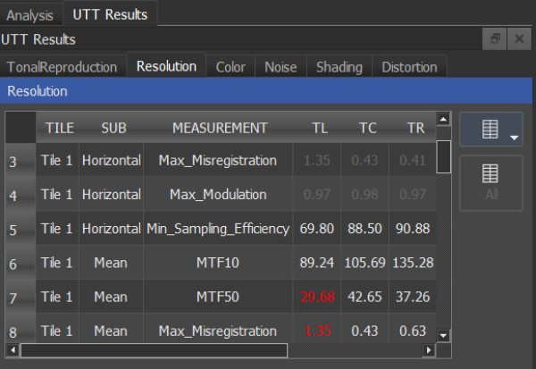
You can easily copy and paste the table to a spreadsheet software for further processing. Just select the cells you want to copy, or click on the top left square to select the entire table. You can also use the context menu which you can open by right-clicking a random cell.

You can also sort the data alphabetically or numerically by clicking on the column header.
Resolution
Resolution is measured on the slanted edges of the UTT Chart. The slanted edges of the tiles have the following names.

All graphs except SFR show a green area, illustrating the specification limits. The bars are within the specification if they are in the green area. Bars outside of the specification area are highlighted in red.
Graphical Results
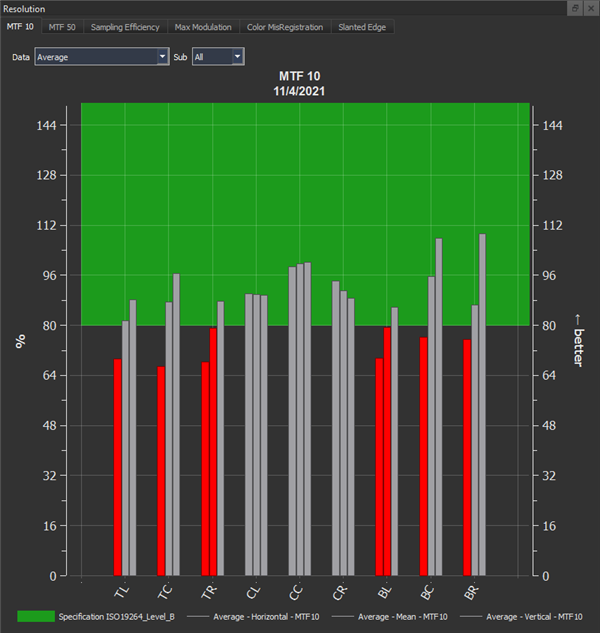
The MTF 10 and MTF 50 plots show each slanted edge's results. The percentage on the y-axis represents the Nyquist Frequency, the maximum frequency the device under test can properly capture. The Nyquist Frequency depends on the pixel resolution of your device. If the bar is not in the green area, meaning the specification, it changes its color to red. A bar can represent the average of the horizontal, vertical, or both edges.
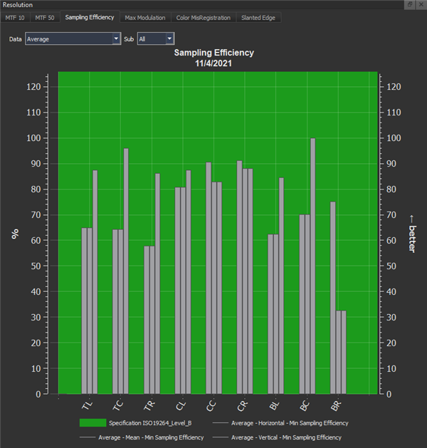
The Sampling Efficiency is the ratio of the limiting resolution, MTF10, and the Nyquist Frequency. If the MTF 10, the spatial frequency at 10% modulation, equals the Nyquist Frequency, the Sampling Efficiency is 100%.
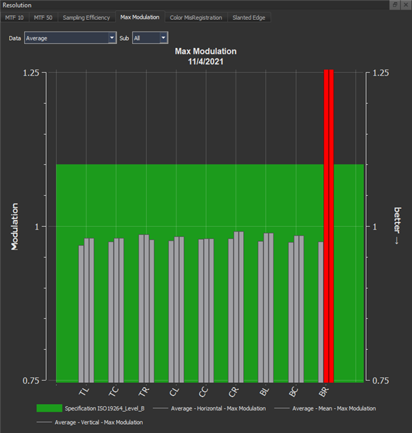
The Max Modulation equals one in an unsharpened image. If sharpening is applied in the image processing of your device, the modulation might be higher; however, it should not exceed the limit defined in the specification.
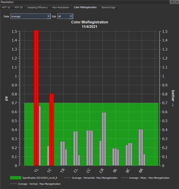
Color Misregistration is the shift of the color channels to each other in px. This shift might be visible in the scan, causing a colored slanted edge. The graphs' bars show the highest Misregistration for horizontal, vertical, or all edges.
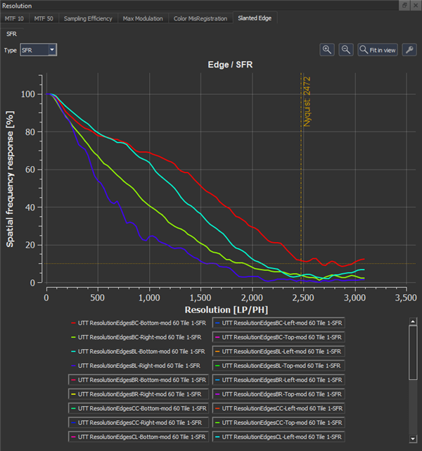
The SFR tab shows all the SFR curves obtained from the slanted edges. In the advanced graph settings, which you can access by clicking the key symbol, you can group the curves to get a better overview.
Numerical Results
MTF10: The spatial frequency ratio with a modulation greater than or equal to 10% to the Nyquist Frequency in percentage.
MTF50: The spatial frequency ratio with a modulation greater than or equal to 50% to the Nyquist Frequency in percentage.
Min_Sampling_Efficiency: If the limiting frequency at 10% modulation equals Nyquist frequency, the sampling efficiency is 100%. The Min_Sampling_Efficiency reflects the lowest Sampling Efficiency of the horizontal, vertical, or all edges.
Max_Modulation: Max_Modulation should be 1 for an unsharpened image. If sharpening is applied in the image processing, the modulation might be higher, but it should not exceed the limit defined in the specification.
Max_MisRegistration: Color Misregistration is the shift of color channels to each other in px. All four edges of a slanted edge patch are analyzed, and the maximum value is taken as the result.
Color
For the Color results, please refer to the chapter color.
Shading
Shading describes the loss of intensity relative to a specified reference in the image. It is measured in all white and gray boxes that are entirely present and can be detected by the software. The detected boxes are marked with a red or blue edge in the image below. As you can see, some of the targets cover the boxes and thus prevent them from being detected.
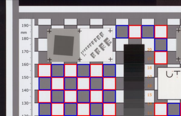
Shading is calculated as the Delta L* in deviation from the mean Delta L* for each box and white and gray boxes separately.
Graphical Results
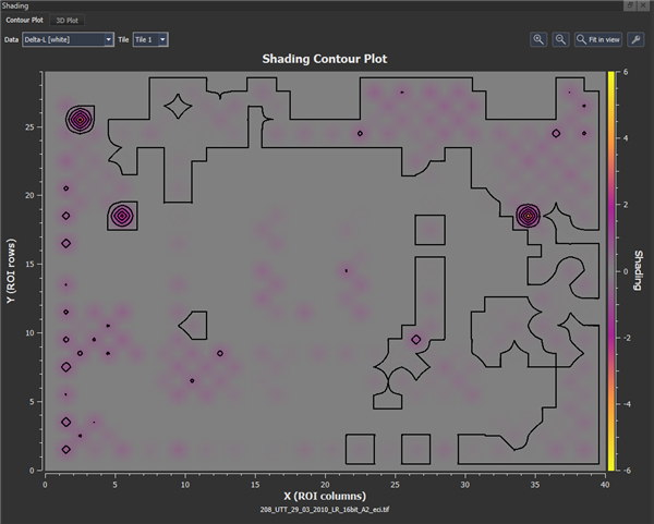
The contour plot shows the Delta L* of the grid's white or gray boxes in the UTT chart. X(ROI rows) and Y(ROI columns) represent the rows and columns of the grid, and the color indicates the deviation value in Delta L*, which can be positive or negative. No deviation is shown in the color gray.
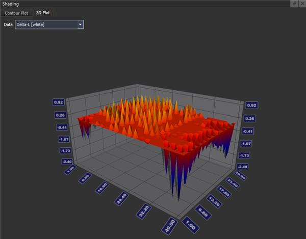
The 3D plot shows the Delta L* of the grid's white or gray boxes in the UTT chart in a three-dimensional view.
Numerical Results
Max_Delta_Gray is the maximum deviation in Delta L* of all gray boxes.
Max_Delta_White is the maximum deviation in Delta L* of all white boxes.
Distortion
Distortion is measured based on all white and gray boxes that are completely present and can be detected, like shading.
The in-between distance of the horizontal and vertical lines is measured in each box (Dist). From there, the average distance of all horizontal and vertical lines of the boxes is determined with sub-pixel accuracy (Dist_mean). The distortion is calculated as the ratio of the distance of each line to the mean distance in percent.
Graphical Results
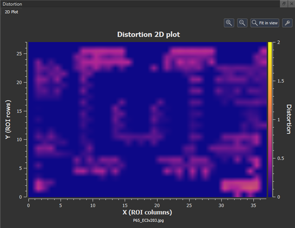
The plot shows the distortion in a color-coded image. The scaling of the color coding can be adjusted in the “Visualization” tab in the “Configuration” dialog. The rows and columns on the Y- and X-Axis represent the white and gray boxes. Note that a distortion value can only be obtained for completely visible boxes.
Numerical Results
Max_Distortion: Max_Distortion is the highest distortion found in all measurements.
Tonal Reproduction
The Tonal Reproduction (also referred to as the opto-electronic conversion function) is measured with the four grayscale targets on the chart. It describes the response of the device under test to the input signal. To achieve an accurate reproduction, the L* values of the sample should be as close as possible to the L* reference values.
Graphical Results
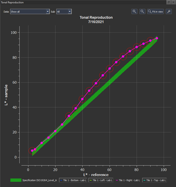 The plot displays the tonal reproduction of the grayscale targets in L* of the sample over L* of the reference. The tile and its four grayscale targets can be selected using the dropdown menus. The tolerance range, defined in the specifications, is displayed in green, and values outside the tolerance range are circled in red.
Numerical Results
Delta_C: The Delta C in between the sample and a specific gray patch reference.
Delta_E: The Delta E in between the sample and a specific gray patch reference.
Lab_L: L* value of the sample.
Additional information regarding L*a*b*, LCh, Delta E, Delta L, Delta C, Delta H: If you express the L*a*b* color space in polar coordinates, you get the LCh space, where L is the luminance, C the chrominance (saturation), and H the hue (color tone). For each of these coordinates, a delta can be determined. The calculation method is defined in the specifications.
White Balance
White balancing is the adjustment of the color channel gains or image processing to achieve a visually neutral reproduction of the input image. It is measured as Delta C or Delta Eab between the sample and reference on the UTT grayscale targets, depending on the specification applied.
Graphical Results
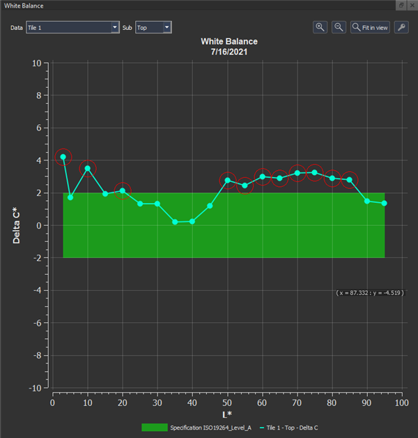
This plot shows the adjustment to keep the grayscale neutral. It shows Delta C over L* of the grayscale targets; at best, Delta C is 0. The specification is displayed in green, and values outside the range are outlined with a red circle.
Numerical Results
Delta C: Delta of C in LCH color space of sample and reference.
Delta E_ab: Delta in “ab” plane of the Lab color space of sample and reference.
Gain Modulation
Gain Modulation describes the reproduction of the tone values of the sample compared to the reference and is measured on the grayscale targets. If Delta L* of sample and reference is equal between two gray patches, the Gain Modulation equals 100%, meaning there is no modulation. A typical example of Gain Modulation is an applied gamma curve.
Example:
| UTT | L* | a* | b* | Delta L | Delta E |
|---|---|---|---|---|---|
| Sample gray patch 1 | 92.59 | -0.88 | -0.12 | ||
| Sample gray patch 2 | 89.82 | -0.74 | 0.82 | 2.77 | 2.93 |
| Reference gray patch 1 | 95 | 0 | 0 | ||
| Reference gray patch 2 | 92 | 0 | 0 | 3 | 3 |
Gain Modulation based on Delta L* is: 2.77 / 3.00 = 0.92 → 92% (OK)
Gain Modulation based on Delta E is: 2.93 / 3.00 = 0.98 → 98% (OK)
Graphical Results
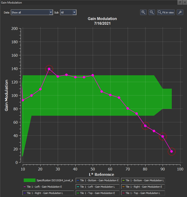
The plot shows the gain modulation based on Delta E or Delta L*. The tolerance range defined in the specifications is displayed in green, and values outside the tolerance range are outlined with a red circle.
Numerical Results
Gain_Modulation_E: Gain Modulation based on Delta E.
Gain_Modulation_L: Gain Modulation based on Delta L.
Noise
Noise is the degradation of a captured image caused by disturbances that are not related to the image signal's actual image content. It can be introduced to a system by the sensor, the quantization, or the image processing. Noise is measured on the single steps of the grayscale targets. The type of Noise measured depends on the specification you apply. In the case of the Metamorfoze specification, Noise equals the sample's standard deviation of L*. ISO19264:2017 contains Noise as “Visual Noise” and considers the Contrast Sensitivity Function and, thus, the human perception of Noise. In version ISO19264:2021 Noise is represented by the RMS of the L* value. For a proper noise measurement, the grayscales must be free from dust, dirt, or scratches.
Graphical Results
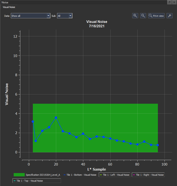
This plot shows the Visual Noise over L* of the gray patches of the sample.
Numerical Results
STD_Dev_DV: This is the standard deviation of Y in digital values in a specific gray patch.
Visual_Noise: Visual Noise is described in ISO 15739. It correlates much better with the human perception of noise than a common SNR measurement.
Lines
The Lines measurement is deactivated by default as it not a requirement of the available standards. You can activate it in the “Analysis Settings” tab under “Analysis”. It helps identify unwanted stripe patterns or banding in an image and is measured on the white, gray, and black horizontal and vertical lines, which are corrected for shading before the measurement.

The relative intensity of the white, black, and gray lines at the upper-horizontal and left-vertical border of each tile over its position is shown in this plot. The specified tolerance is displayed in green, and values out of specification are marked with a red circle.
Export of Results
You can export the results as a .xml file or a .pdf under “Export analysis” in the “File” menu. If you select .pdf, choose “UTT Overview” if you only want a basic report with pass or fail information, choose “UTT Full” if you want to export the entire results. Only the measurements which are checked will be included in the report.
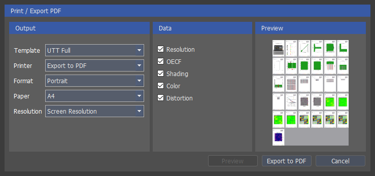
The .xml file includes all measurements as numerical values.
UTT Settings
The settings are automatically assigned according to the selected standard, but you can change it manually by activating “Overide default settings from standards”. The Metamorfoze standards require CIE 1976 as the color difference formula, and “Gain Modulation Expanded” has to be deactivated. For ISO19264, “Gain Modulation Expanded” has to be activated, and the color difference formula is CIE2000 SL1. Note, that you have to save the changes to the settings first, before you can assign it to an analysis.
| Standard | Gain Modulation Expanded | Color Difference Formula |
|---|---|---|
| ISO19264 | on | CIE2000 SL1 |
| Metamorfoze | off | CIE 1976 |
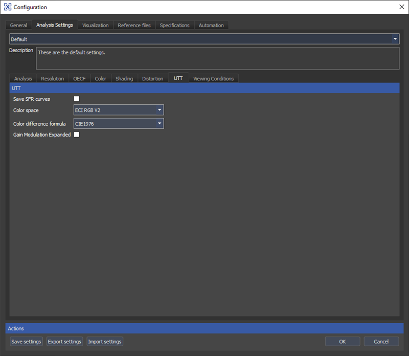
Save SFR Curves
Activate this option to save all SFR curves to the database.
Color Difference Formula
Select the Color Difference Formula you want to apply for calculating Delta E, Delta L, and other metrics. More details about the formulas are stated in the Color section.
Color Space
This setting only applies if you have selected “Embedded profile” as the color profile during image import, but the color profile cannot be read. In that case, the selected color space is used for the analysis.
Gain Modulation Expanded
If selected, the L* spacing of two patches is used to calculate the gain modulation instead of a one-step spacing.
Metric Selection
In the “Analysis” tab select the metrics you want to include in your measurement and save it to your analysis settings.

Automation
Two options are available to automate the image quality analysis, “Hot folders” or “Command Line.” A “Hot Folder” is a folder in which you can copy your test images for processing. All images in the folder are queued and then processed using the analysis settings you set for the folder. Use “Command Line” in the Windows Command Line Interface(CLI) to execute specific commands. A more convenient way to use command lines is to create a batch file. IQ-Analyzer-X provides a dialog to generate a simple batch file, so you do not need to start from scratch.
Hot Folders
To create a “Hot Folder,” go to the “Automation” tab in the “Configuration” dialog. Click on the “Hot folders” and then the “Settings” tab to show a list of the “Observed folders” and their settings.
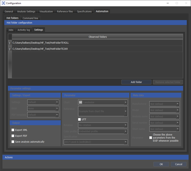
You can add and remove folders from the “Observed folders” list in the “Settings” tab. Each folder can have an individual configuration. For example, one folder could be for TE269 analysis and another for TE42LL, each with different analysis settings. To change the configuration of a folder, select it in the list; the selected folder will be highlighted. Note that you must first select an “Output” option to establish other settings. You can choose between “Export XML,” “Export PDF,” and “Save analysis automatically” as an output. “Save analysis automatically” saves the analysis in the connected database. All required settings are available once the checkbox is activated.
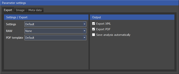
Under the “Image” tab you find all settings from the regular image import dialog. Check the UTT checkbox and select the desired specification in case you want to analyze a UTT.
UTT users only: Note, that you currently need to assign a chart layout ( UTT_A0, UTT_A1, UTT_A2, UTT_A3 or UTT_A4) manually, as there is no automatic chart detection for UTT.
If you set “Reference” to “automatic”, iQ-Analyzer-X will assign the most suitable reference file to the chart in terms of capture date and reference file validity. For example, if the capture date of the image is August 2023, it will choose the reference file valid in this period.
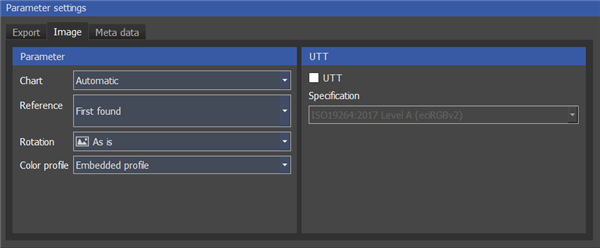
Provide information about the test images in the “Metadata” tab.
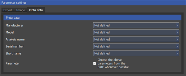
This information is used to save the analysis into the database or to name the PDF/XML file. Providing as much information as possible will help you find the analysis later in the database. Note that you do not need to enter an actual manufacturer or device model. You can also come up with names that fit your concept. If you check “Choose the above parameters from EXIF whenever possible,” the software uses EXIF data if available.
If all required information is provided, change to the “Activity log” or “Jobs” tab to activate the “Hot folder” with the “Activate” button.
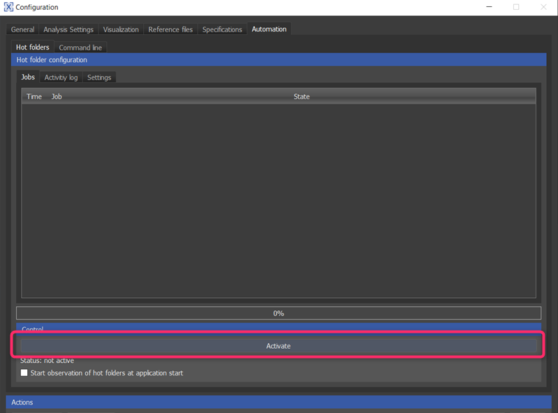
Once the hot folder is activated, all images copied here are analyzed subsequently. The results are saved either into your database if you have selected “Save analysis automatically” or in a subfolder called “output” if you selected “Export XML” or “Export PDF.” In the subfolder you can also find the “checkimages”, which show the detected ROIs. While the hot folder is activated, the software’s main window disappears and reappears as soon as it is deactivated. For convenience, activating the relevant checkbox can activate the “Hot folders” directly at the start-up of iQ-Analyzer-X.
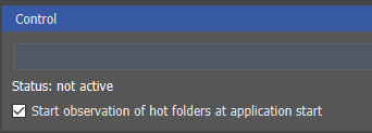
During the next software start-up, only the “Automation” tab is seen, and the “Hot folder” is active immediately. Deactivate the “Hot Folder” to close the software after you finish.
We recommend zipping the image files first if you have plenty of images to process. Copy this zip file to the hot folder to process all images in the container.
Command Line
Create a batch file
The advantage of creating a batch file is your ability to process multiple commands with a simple double-click. In the “Command Line” tab under “Automation,” you can create a batch file that you can use to develop more complex procedures. The batch file can be edited with a standard text editor. Note that all commands must be in the same row to be processed correctly.
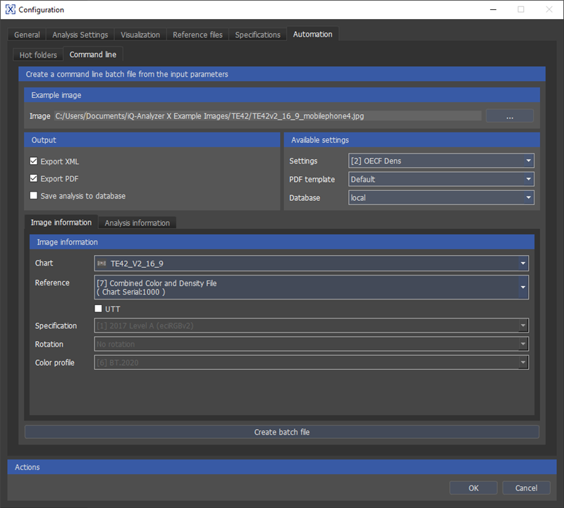
First, load an example image similar to the ones you want to process. Then enter all required information in the “Output” and “Available settings” sections and the “Analysis Information” and “Image Information” tabs. Once done, click on “Create batch file.” You can now save the file in your desired location.
The commands in the list below are available to extend the functionality of your batch file. You can use the regular command with “- -“ or a short command with a single ”-“ before it. Some commands, e.g., “reference,” require an ID. The IDs are shown in brackets in the relevant dropdown menu entry of the command line tab.


| Command | Short command | Available Arguments | Description | Example |
|---|---|---|---|---|
| chart | c | “TheChartname” | The captured chart in all images | --chart="TE42_V2_16_9" |
| database | “local”, “YourDatabaseName” | The name of the database | --database="local" |
|
| enableMRE | - | - | Enable manual ROI editing in command line mode | --enableMRE |
| manufacturer | m | “YourManufacturer” or “Unknown” | The name of the camera manufacturer | --manufacturer="ExampleManufacturer" |
| model | - | “YourModel” | The model of the camera | --model="ExampleModel" |
| name | - | “YourAnalysisName” | The name of the analysis | --name="TE42LL_Lowlight_Test" |
| orientation | o | 0, 90, 180, 270 | The image orientation in degrees | --orientation=180 |
| p | “YourResultPDFPath+FileName” | Export result as PDF file | --pdf="C:/Users/Documents/TE42v2_16_9_mobilephone4_Report.pdf" |
|
| preferExif | i | - | Prefer EXIF meta data for analysis | --preferExif |
| profile | l | “Embedded profile”, “Adobe RGB”, “sRGB”, “ECI RGB V2”, “Display P3”, “BT.2020” | The color profile | --profile="Adobe RGB" |
| reference | r | “YourReferenceID” | The ID of the reference file | --reference="5" |
| rois | - | “YourPathToROIs+FileName” | The path to the .xml file, which contains the ROIs | --rois="C:/Users/ADent/Desktop/MyROIs.xml" |
| save | v | - | Save analysis to database | --save |
| serial | - | “YourSerial” | The serial number of the camera | --serial="123456" |
| settingsID | s | settings ID as integer number | Defines the settings set used for this analysis by it's ID | --settingsID=1 |
| shortname | v | “YourShortName” | The short name of the analysis | --shortname="ExampleShortname" |
| specification | - | “YourSpecificationID” | The specification ID to be used with UTT charts | --specification="4" |
| template | t | “Default”, “UTT_Overview” , “UTT_Full” | Define the template for PDF export | --template="Default" |
| utt | u | - | Make UTT analysis | --utt |
| xml | x | “YourResultXMLPath+FileName” | Export result as XML file | --xml="C:/Users/User/Documents/Images/TE42v2_16_9_mobilephone4_Results.xml" |
CLI for UTT
UTT requires some special calls when working with CLI.
If a UTT image is analyzed, the -u or –UTT parameter must be set.
The correct chart must be specified, as no automatic chart classification takes place with UTT.
If a *.pdf export is required, a UTT template must be selected for the Template parameter (either “UTT_Overview” or “UTT_Full”)
Example Batch Files
This is a simple batch file created with iQ-Analyzer-X that runs an analysis on a TE42 V2 .jpg image and saves a .xml and .pdf file with the results. Note, that the path to iQ-Analyzer-X.exe, the path to the image and the commands need to be in the same row. The format in this example is only for a better overview.
"C:/Program Files/Image Engineering/iQ-Analyzer-X 1.x.x/iQ-Analyzer-X.exe" "C:/Users/User/Documents/TE42/TE42v2_16_9_mobilephone4.jpg"
--settingsID=1
--reference="7"
--template="Default"
--chart="TE42_V2_16_9"
--xml="C:/Users/User/Documents/TE42/TE42v2_16_9_mobilephone4.xml"
--pdf="C:/Users/User/Documents/TE42/TE42v2_16_9_mobilephone4.pdf"
--manufacturer="ExampleManufacturer"
--model="ExampleModel"
--name="ExampleName"
--serial="ExampleSerial"
--shortname="ExampleShortname"
--preferExif
This is a batch file that analyzes multiple .jpg images of a TE42 V2 and saves a .xml and .pdf file with the results.
"C:/Program Files/Image Engineering/iQ-Analyzer-X 1.x.x/iQ-Analyzer-X.exe"
"C:/Users/User/Documents/IE/iQ-Analyzer Bilder/TE42/canm200_te42v2_iso100.JPG"
"C:/Users/User/Documents/IE/iQ-Analyzer Bilder/TE42/canm200_te42v2_iso200.JPG"
"C:/Users/User/Documents/IE/iQ-Analyzer Bilder/TE42/canm200_te42v2_iso400.JPG"
"C:/Users/User/Documents/IE/iQ-Analyzer Bilder/TE42/canm200_te42v2_iso800.JPG"
"C:/Users/User/Documents/IE/iQ-Analyzer Bilder/TE42/canm200_te42v2_iso1600.JPG"
"C:/Users/User/Documents/IE/iQ-Analyzer Bilder/TE42/canm200_te42v2_iso3200.JPG"

--settingsID=1
--settingsID=2
--settingsID=3
--settingsID=2
--settingsID=2
--settingsID=1

--reference="-1"
--template="Default"
--xml="C:/Users/User/Documents/IE/iQ-Analyzer Bilder/TE42/canm200_te42v2_iso1600.xml"
--pdf="C:/Users/User/Documents/IE/iQ-Analyzer Bilder/TE42/canm200_te42v2_iso1600.pdf"
--manufacturer="Canon"
--model="EOS 200D"
--name="canm200_te42v2_iso1600.JPG"
--serial="56786543"
--shortname="Automationtest"
--preferExif
When you double-click a batch file, iQ-Analyzer-X starts from the command line and shows up in the taskbar. You can observe the processing of the images in the iQ-Analyzer-X window. When the analysis is finished, the CLI and the iQ-Analyzer-X window close automatically. If you do not save in the database, the .pdf or .xml results are saved in the provided path. A folder with the check images is created in the folder of the analyzed image. In the check image you can see, if all the ROIs were set properly.
Custom Chart Layouts
If you have ordered a custom chart from Image Engineering that can be analyzed by iQ-Analyzer-X, you will receive a chart file (*.chart) and the corresponding reference file (*.ref). The *.chart file contains information about the layout with its targets, and the reference file contains the color and/or density values.
Copy the *.chart file into the “charts” folder of the iQ-Analyzer-X version you want to use.
C:\Program Files\Image Engineering\iQ-Analyzer-X…\resources\charts
Note, that it has to be copied again, if you update iQ-Analyzer-X.
Import the reference file as described in the chapter "Reference Files" .
The reference file will be imported in the database and is not affected by future updates.
Note that if you want to analyze a custom chart, the automatic recognition won't work because it is not trained for custom charts. If this happens often, you can disable automatic chart classification in the “General” tab in the configuration dialog.
Abbreviations
CH - Cultural Heritage
DUT - Device under Test
DV - Digital Value
GUI - Graphical User Interface
LCA - Longitudinal Chromatic Aberration
LGD - Lens Geometric Distortion
LP - Linepairs
MTF - Modulation Transfer Function
OECF - Opto Electronic Conversion Function
PH - Picture Height
PX - Pixel
ROI - Region of Interest
SFR - Spatial Frequency Response
SNR - Signal-to-Noise Ratio
Troubleshooting
In the event of any technical issues, please contact image engineering support.
Phone
+49 2273 99 99 1-60
Email
support@image-engineering.de
Please remember to provide your version number. If you are having trouble analyzing an image, please send the image of concern with the iQ-Analyzer.log file. The file is located here:
C:\Users\YourUserName\AppData\Roaming\Image Engineering\iQ-Analyzer-X
Thanks for your help!
Regulations
Copyright
End user license agreement (EULA)
1 PREAMBLE
This Agreement governs the relationship between Licensee, a Business Entity, (hereinafter: Licensee) and Image Engineering GmbH & Co. KG, a duly registered company in whose principal place of business is Im Gleisdreieck 5, 50169 Kerpen-Horrem, Germany (hereinafter: Image Engineering). This Agreement sets the terms, rights, restrictions and obligations on using iQ-Analyzer-X (hereinafter: The Software) created and owned by Image Engineering, as detailed herein.
2 SOFTWARE PROTECTION
Image Engineering maintains its right to protect its intellectual property by using modern advances in software protection against un-authorized use and software piracy.
Along with The Software, Licensee of the professional version will receive a dongle that will serve as a security measure to enable Licensee’s use of The Software (hereinafter: Dongle). In order to use The Software, the Dongle must at all times while using the software remain connected to the hardware on which The Software is installed. Licensee acknowledges and agrees that The Software will not function properly if Dongle is removed from such hardware.
3 LICENSE GRANT
Image Engineering hereby grants Licensee a limited, non-assignable and non-sub licensable, perpetual, commercial, non-exclusive license, all in accordance with the terms set forth and other legal restrictions set forth in 3rd party software used while running the Software.
4 PERMITTED USES
4.1 INSTALLATION
Licensee may install and use the number of copies of The Software that Licensee has purchased or has been granted a license for. If The Software is protected by Dongle, Licensee may install unlimited number of copies of The Software but only use The Software on the hardware with the attached Dongle.
4.2 SERVER DEPLOYMENT
Licensee may install one copy of the professional version of The Software on an internal file server for purposes of downloading and installing The Software on licensed computers within the same internal network.
4.3 BACKUP AND ARCHIVAL COPIES
Licensee may make copies of the professional version of The Software solely for backup or archival purposes. Licensee agrees to maintain records of the location and use of each copy, in whole or in part. Each copy of The Software is copyrighted but unpublished by Image Engineering. Licensee agrees to reproduce and apply the copyright notice and proprietary notice of Image Engineering to all copies made hereunder, in whole or in part and in any form, of The Software.
4.4 PUBLISHING
Licensee may use and publish the output of The Software to 3rd parties.
5 PROHIBITED USES
5.1 REVERSE ENGINEERING
Licensee is not permitted to decompile, disassemble, reverse engineer, or otherwise attempt to derive the source code for any version of The Software.
5.2 TRANSFER TO A 3RD PARTY
Licensee is not permitted to rent, lease or redistribute The Software. Licensee may not provide or otherwise make available The Software or any copy in whole or in part, whether modified or unmodified, to any person other than employees of Licensee without the prior explicit written consent of Image Engineering.
6 PROPRIETARY RIGHTS
Licensee is not permitted to alter, remove or circumvent the intellectual property right notices on the software product including the documentation, particularly the copyright notices or trademarks. Licensee is permitted to share the information how and where to download The Software on Image Engineering’s website. But Licensee is not permitted to share the software with other people except those necessary to install the software on Licensee’s computer nor is he allowed to distribute the software in any way. Licensee recognizes that Image Engineering regards The Software as its proprietary information and as confidential trade secrets of great value. Licensee further agrees to treat the Licensed Programs with at least the same degree of care with which Licensee treats its own confidential information and in no event with less care than is reasonably required to protect the confidentiality of The Software.
7 TERM AND TERMINATION
7.1 TERM This License Agreement is effective upon installation of The Software and will continue in force until terminated.
7.2 TERMINATION
a) Licensee Right of Termination: Licensee may terminate the Agreement at any time by destroying all copies of The Software and in case of the professional version additionally the Dongle.
b) Image Engineering Right of Termination: Image Engineering may terminate this Agreement if Licensee violates any of the terms and conditions of this Agreement and fails to correct such violation within ten (10) days after receiving written notice thereof from Image Engineering.
c) Effect of Termination: In the event of termination, Licensee will immediately discontinue use of The Software. Within one (1) month after termination of this Agreement, Licensee will furnish a certificate to Image Engineering which certifies that, through its best effort and to the best of its knowledge, the original and all copies, in whole or in part and in any form, of The Software have been destroyed.
8 PAYMENT
In consideration of the License granted under clause 3 “License Grant”, Licensee shall pay Image Engineering a fee for the professional version of The Software, via any mean which Image Engineering may deem adequate. Failure to perform payment shall construe as material breach of this Agreement. License fees do not include any shipping, duties, bank fees, sales, use, excise or similar taxes due.
9 UPGRADES, UPDATES AND FIXES
Image Engineering may provide Licensee, from time to time, with Upgrades, Updates or Fixes, as detailed herein and according to his sole discretion. Licensee hereby warrants keeping The Software up-to-date and installing all relevant updates and fixes, and may, at his sole discretion, purchase upgrades, according to the rates set by Image Engineering. Nothing in this Agreement shall require Image Engineering to provide Updates or Fixes.
9.1 UPGRADE
For the purpose of this license, an Upgrade shall be a material amendment in The Software, which contains new features and or major performance improvements and shall be marked as a new version number. For example, should Licensee purchase The Software under version 1x.x, an upgrade shall commence under number 2.0.0.
9.2 UPDATE
For the purpose of this license, an update shall be a minor amendment in The Software, which may contain new features or minor improvements and shall be marked as a new sub-version number. For example, should Licensee purchase The Software under version 1.1.x, an upgrade shall commence under number 1.2.0.
9.3 FIX
For the purpose of this license, a fix shall be a minor amendment in The Software, intended to remove bugs or alter minor features which impair The Software's functionality. A fix shall be marked as a new sub-sub-version number. For example, should Licensee purchase The Software under version 1.1.1, an upgrade shall commence under number 1.1.2.
10 MAINTENANCE
By purchasing The Software, Licensee is granted a one-year standard membership in the Maintenance program (hereinafter: The Maintenance) at no extra charge. The Maintenance is not automatically extended. The optional extension of The Maintenance will involve additional costs. If the maintenance is not extended within three (3) months after the day of expiration, an additional re-entry fee of sixty percent (60%) of the maintenance costs is applied within the first twelve (12) months after the initial expiration date. Once the maintenance has been expired for over twelve (12) months, one hundred percent (100%) of the maintenance will be applied in addition to the maintenance costs. In the event that the maintenance has been expired over twenty-four (24) months, re-entry can only be offered if a new license of the iQ-Analyzer-X is purchased.
10.1 STANDARD MAINTENANCE
Standard Maintenance includes following privileges at no additional charge:
a) Upgrades of The Software according to clause 9.1 “Upgrade” (if The Maintenance has expired, upgrades of The Software must be purchased under the usual conditions without any discount)
b) Telephone Support
c) E-Mail support
d) Attendance at regularly offered webinars
e) Supply of chart layout and a reference data files for one (1) custom-made chart per year (the manufacturing of the chart may involve additional costs). The chart layout is considered as “final with no additional modifications required” if the Licensee can analyse a set of images that was provided to Image Engineering showing the custom made chart for the creation process. Image Engineering might refuse additional modifications or provide these modifications on a payed basis only after the status “final” was reached.
10.2 ADVANCED MAINTENANCE
Advanced Maintenance includes following privileges at no additional charge:
a) Upgrades of The Software according to clause 9.1 “Upgrade” (if The Maintenance has expired, upgrades of The Software must be purchased under the usual conditions without any discount)
b) Telephone Support
c) E-Mail support
d) Attendance at regularly offered webinars
e) Supply of chart layout and a reference data files for up to five (5) custom-made charts per year (the manufacturing of the charts may involve additional costs). The chart layout is considered as “final with no additional modifications required” if the Licensee can analyse a set of images that was provided to Image Engineering showing the custom made chart for the creation process. Image Engineering might refuse additional modifications or provide these modifications on a payed basis only after the status “final” was reached.
f) Supply of reference data for up to five (5) individually measured charts.
g) Two (2) days training course with Licensee specific content. Online training courses and training courses at Image Engineering’s office are provided at no additional charge. For training courses at Licensee’s location, all travel and accommodation expenses shall be borne by Licensee.
11 SUPPORT
The Software is provided with limited support. Image Engineering shall provide support via electronic mail and on regular business days and hours, German time.
11.1 BUG NOTIFICATION
Licensee may provide Image Engineering of details regarding any bug, defect or failure in The Software promptly and with no delay from such event. Licensee shall comply with Image Engineering's request for information regarding bugs, defects or failures and furnish him with information, screenshots and try to reproduce such bugs, defects or failures.
11.2 FEATURE REQUEST
Licensee may request additional features in The Software, provided, however, that
a) Licensee shall waive any claim or right in such feature should feature be developed by Image Engineering;
b) Licensee shall be prohibited from developing the feature, or disclose such feature request, or feature, to any 3rd party directly competing with Image Engineering or any 3rd party which may be, following the development of such feature, in direct competition with Image Engineering;
c) Licensee warrants that feature does not infringe any 3rd party patent, trademark, trade-secret or any other intellectual property right;
d) Licensee developed, envisioned or created the feature solely by himself.
Image Engineering will consider such feature requests for future versions and shall only be bound to the development of such feature in case of a written additional agreement between Liecensee and Image Engineering. Such an agremement may be subject to additional costs.
12 REPLACEMENT POLICY FOR DAMAGED, LOST AND STOLEN DONGLES
12.1 DEFECTIVE DONGLE (LICENSEE WITH CURRENT MAINTENANCE)
If a Dongle fails or becomes defective, it may be replaced as follows:
a) There are no fees for the replacement of a defective Dongle unless the defect is caused by force or careless or improper use of the Dongle.
b) Licensee shall return the defective Dongle to Image Engineering by registered mail as soon as possible, but not later than three (3) months after express written declaration of damage. Once the Dongle has been received by Image Engineering, a replacement Dongle will be issued with the corresponding license to authorize the software products that are covered under the current maintenance contract for the Dongle being replaced.
c) If Licensee fails to return the defective Dongle within the allotted time period, Image Engineering, in its sole discretion, may refuse the replacement.
12.2 DEFECTIVE DONGLE (LICENSEE WITH EXPIRED MAINTENANCE)
If a Dongle fails or becomes defective, it may be replaced as follows:
a) Licensee shall pay Image Engineering a fee of 200.00 EUR for the replacement of a defective Dongle.
b) Licensee shall contact Image Engineering for a sales quotation for a replacement Dongle. The sales quotation is to be used to generate a purchase order for the necessary amount plus any applicable costs, i.e. taxes and shipping. the purchase order or required form of payment
c) Licensee shall return the defective Dongle to Image Engineering by registered mail as soon as possible together with the purchase order or required form of payment. Once the Dongle and purchase order have been received by Image Engineering, a replacement Dongle will be issued with the corresponding license to authorize the software products that are covered under the current maintenance contract for the Dongle being replaced.
d) If Licensee fails to return the defective Dongle within the allotted time period, Image Engineering, in its sole discretion, may refuse the replacement.
12.3 LOST OR STOLEN DONGLE
If a Dongle is lost or stolen the following shall apply:
a) Licensee shall contact Image Engineering without undue delay to notify Image Engineering that the Dongle is no longer in its possession.
b) Licensee shall pay Image Engineering a penalty fee in the amount of ten (10) percent of the current list price of the lost or stolen license without any discount plus any applicable costs, i.e. taxes and shipping.
c) When Image Engineering receives the penalty fee payment, the replacement Dongle will be shipped to the Licensee.
d) If a Dongle reported as lost or stolen is found after the replacement Dongle has been shipped to Licensee, Licensee shall return it to Image Engineering without undue delay.
e) If a Dongle reported as lost or stolen is used again for any reason at any location, Licensee shall pay Image Engineering a penalty fee in the amount of two hundred (200) percent of the current list price of the license in use without any discount.
13 LIABILITY
The Software is provided under an “AS-IS” basis. Image Engineering shall never, and without any limit, be liable for any damage, cost, expense or any other payment (including, without limitation, incidental, direct, indirect, special or consequential damages, damages for loss of business profits, business interruption, loss of business information, or other pecuniary loss) incurred by Licensee as a result of Software’s actions, failure, bugs and/or any other interaction between The Software and Licensee’s end-equipment, computers, other software or any 3rd party, end-equipment, computer or services. Moreover, Image Engineering shall never be liable for any defect in source code written by Licensee when relying on The Software.
14 WARRANTY
Considerable time, effort and expense have gone into the development of The Software, and it has been thoroughly tested and used. However, except as otherwise specifically provided herein, no warranty is made on its accuracy or reliability. It is the responsibility of the Licensee to verify the results obtained from The Software. In the event The Software is found to be defective, Image Engineering's only obligation is to remedy the defect. Image Engineering will in no event have obligations or liabilities for incidental or consequential damages associated with the use of The Software.
14.1 INTELLECTUAL PROPERTY
Image Engineering hereby warrants that The Software does not violate or infringe any 3rd party claims in regards to intellectual property, patents and/or trademarks and that to the best of its knowledge no legal action has been taken against it for any infringement or violation of any 3rd party intellectual property rights.
14.2 NO-WARRANTY
The Software is provided without any warranty. Image Engineering hereby disclaims any warranty that The Software shall be error free, without defects or code which may cause damage to Licensee’s computers or to Licensee, and that The Software shall be functional. Licensee shall be solely liable to any damage, defect or loss incurred as a result of operating The Software and undertake the risks contained in running The Software on Licensee’s computer system(s).
14.3 PRIOR INSPECTION
Licensee hereby states that he inspected The Software thoroughly and found it satisfactory and adequate to his needs, that it does not interfere with his regular operation and that it does meet the standards and scope of his computer systems and architecture. Licensee found that The Software interacts with his environment and that it does not infringe any of End User License Agreement of any software Licensee may use in performing his services. Licensee hereby waives any claims regarding The Software's incompatibility, performance, results and features, and warrants that he inspected The Software.
15 NO REFUNDS
Licensee warrants that he inspected The Software according to clause 14.3 “Prior Inspection” and that it is adequate to his needs. Accordingly, as The Software is intangible goods, Licensee shall not be, ever, entitled to any refund, rebate, compensation or restitution for any reason whatsoever, even if The Software contains material flaws.
16 INDEMNIFICATION
Licensee hereby warrants to hold Image Engineering harmless and indemnify Image Engineering for any lawsuit brought against it in regards to Licensee’s use of The Software in means that violate, breach or otherwise circumvent this license, Image Engineering's intellectual property rights or Image Engineering's title in The Software. Image Engineering shall promptly notify Licensee in case of such legal action and request Licensee’s consent prior to any settlement in relation to such lawsuit or claim.
17 GOVERNING LAW, JURISDICTION
Licensee hereby agrees not to initiate class-action lawsuits against Image Engineering in relation to this license and to compensate Image Engineering for any legal fees, cost or attorney fees should any claim brought by Licensee against Image Engineering be denied, in part or in full. The governing law for this agreement shall be the law of Germany with the place of jurisdiction being Cologne, Germany.
18 SEVERABILITY
If any provision or provisions of this Agreement shall be held to be invalid, illegal, unenforceable or in conflict with the law of any jurisdiction, the validity, legality and enforceability of the remaining provisions shall not in any way be affected or impaired thereby.
Trademarks
Microsoft® and Windows® are either registered trademarks or trademarks of Microsoft Corporation in the United States and/or other countries.
Third party tools
The iQ-Analyzer-X uses open source as well as commercial software and libraries.
Armadillo
Armadillo C++ Linear Algebra Library is licensed under the Apache License 2.0
Copyright 2008-2020 Conrad Sanderson
Copyright 2008-2016 National ICT Australia (NICTA)
Copyright 2017-2020 Arroyo Consortium
Copyright 2017-2020 Data61, CSIRO
This product includes software developed by Conrad Sanderson
This product includes software developed at National ICT Australia (NICTA)
This product includes software developed at Arroyo Consortium
This product includes software developed at Data61, CSIRO
Dlib
Boost Software License - Version 1.0 - August 17th, 2003
Permission is hereby granted, free of charge, to any person or organization obtaining a copy of the software and accompanying documentation covered by this license (the “Software”) to use, reproduce, display, distribute, execute, and transmit the Software, and to prepare derivative works of the Software, and to permit third-parties to whom the Software is furnished to do so, all subject to the following:
The copyright notices in the Software and this entire statement, including the above license grant, this restriction and the following disclaimer, must be included in all copies of the Software, in whole or in part, and all derivative works of the Software, unless such copies or derivative works are solely in the form of machine-executable object code generated by a source language processor.
THE SOFTWARE IS PROVIDED “AS IS”, WITHOUT WARRANTY OF ANY KIND, EXPRESS OR IMPLIED, INCLUDING BUT NOT LIMITED TO THE WARRANTIES OF MERCHANTABILITY, FITNESS FOR A PARTICULAR PURPOSE, TITLE AND NON-INFRINGEMENT. IN NO EVENT SHALL THE COPYRIGHT HOLDERS OR ANYONE DISTRIBUTING THE SOFTWARE BE LIABLE FOR ANY DAMAGES OR OTHER LIABILITY, WHETHER IN CONTRACT, TORT OR OTHERWISE, ARISING FROM, OUT OF OR IN CONNECTION WITH THE SOFTWARE OR THE USE OR OTHER DEALINGS IN THE SOFTWARE.
dcraw
Copyright © 1997-2015 by Dave Coffin
This is free software.
Web site of the author: http://www.dechifro.org/index.html
The documentation can be found here: http://www.dechifro.org/dcraw/dcraw.1.html
ExifTool
Copyright © 2003-2020 by Phil Harvey
This is free software. It is licensed under the same terms as Perl itself: https://dev.perl.org/licenses
The documentation can be found here: https://exiftool.org
You can download the complete source code here: https://github.com/exiftool/exiftool
libexif
The libexif C EXIF library
Is licensed under the GNU LESSER GENERAL PUBLIC LICENSE Version 2.1 (LGPL).
Little CMS
Little CMS Open Source Color Engine
License: MIT License
To the question, Is this software really free? as long as you abide by the licensing conditions, yes. It is free under the MIT license agreement. You can use Little CMS in your commercial apps, too. The license requires a pointer referencing the copyright, so you can add a file in your distribution disk saying that your product uses Little CMS, and the copyright notice. That’s all. Of course, if you use the package and can improve on it, then your contribution will be welcome, but please note this is not required. However, you should consider the maintenance overhead of keeping your own custom version of Little CMS, versus the advantages you might get from participating in the community, such as bugfixes and extensions that others may make on top of yours.
OpenCV
License Agreement For Open Source Computer Vision Library (3-clause BSD License)
Copyright (C) 2000-2020, Intel Corporation, all rights reserved.
Copyright (C) 2009-2011, Willow Garage Inc., all rights reserved.
Copyright (C) 2009-2016, NVIDIA Corporation, all rights reserved.
Copyright (C) 2010-2013, Advanced Micro Devices, Inc., all rights reserved.
Copyright (C) 2015-2016, OpenCV Foundation, all rights reserved.
Copyright (C) 2015-2016, Itseez Inc., all rights reserved.
Copyright (C) 2019-2020, Xperience AI, all rights reserved.
Third party copyrights are property of their respective owners.
Redistribution and use in source and binary forms, with or without modification, are permitted provided that the following conditions are met:
- Redistributions of source code must retain the above copyright notice, this list of conditions and the following disclaimer.
- Redistributions in binary form must reproduce the above copyright notice, this list of conditions and the following disclaimer in the documentation and/or other materials provided with the distribution.
- Neither the names of the copyright holders nor the names of the contributors may be used to endorse or promote products derived from this software without specific prior written permission.
This software is provided by the copyright holders and contributors “as is” and any express or implied warranties, including, but not limited to, the implied warranties of merchantability and fitness for a particular purpose are disclaimed. In no event shall copyright holders or contributors be liable for any direct, indirect, incidental, special, exemplary, or consequential damages (including, but not limited to, procurement of substitute goods or services; loss of use, data, or profits; or business interruption) however caused and on any theory of liability, whether in contract, strict liability, or tort (including negligence or otherwise) arising in any way out of the use of this software, even if advised of the possibility of such damage.
QsLog
Copyright © 2014, Razvan Petru
All rights reserved.
Redistribution and use in source and binary forms, with or without modification, are permitted provided that the following conditions are met:
- Redistributions of source code must retain the above copyright notice, this list of conditions and the following disclaimer.
- Redistributions in binary form must reproduce the above copyright notice, this list of conditions and the following disclaimer in the documentation and/or other materials provided with the distribution.
- The name of the contributors may not be used to endorse or promote products derived from this software without specific prior written permission.
THIS SOFTWARE IS PROVIDED BY THE COPYRIGHT HOLDERS AND CONTRIBUTORS “AS IS” AND ANY EXPRESS OR IMPLIED WARRANTIES, INCLUDING, BUT NOT LIMITED TO, THE
IMPLIED WARRANTIES OF MERCHANTABILITY AND FITNESS FOR A PARTICULAR PURPOSE ARE DISCLAIMED.
IN NO EVENT SHALL THE COPYRIGHT HOLDER OR CONTRIBUTORS BE LIABLE FOR ANY DIRECT, INDIRECT, INCIDENTAL, SPECIAL, EXEMPLARY, OR CONSEQUENTIAL DAMAGES
(INCLUDING,BUT NOT LIMITED TO, PROCUREMENT OF SUBSTITUTE GOODS OR SERVICES; LOSS OF USE,DATA, OR PROFITS; OR BUSINESS INTERRUPTION) HOWEVER CAUSED AND
ON ANY THEORY OF LIABILITY, WHETHER IN CONTRACT, STRICT LIABILITY, OR TORT (INCLUDING NEGLIGENCE OR OTHERWISE) ARISING IN ANY WAY OUT OF THE USE OF THIS
SOFTWARE, EVEN IF ADVISED OF THE POSSIBILITY OF SUCH DAMAGE.
The source code is available here:
https://github.com/victronenergy/QsLog
Qt
The Qt framework is licensed under the commercial Qt license.
Qwt
The Qwt library contains GUI Components and utility classes which are primarily useful for programs with a technical background. Beside a framework for 2D plots it provides scales, sliders, dials, compasses, thermometers, wheels and knobs to control or display values, arrays, or ranges of type double.
Qwt is distributed under the terms of the Qwt License, Version 1.0.
QwtPolar
The QwtPolar library contains classes for displaying values on a polar coordinate system.
QwtPolar is distributed under the terms of the Qwt License, Version 1.0.
TensorFlow
C API for TensorFlow.
Licensed under the Apache License, Version 2.0
